Sequence Analysis¶

Loading a Reference¶

When analysing the outcome of a protein design set, it can be useful to retrieve the data from the source structure (template) in order to assess, on a sequence level, which changes have happened.

For the purpose of this example, we will use a domain from a Putative formate dehydrogenase accessory protein. To load the data, we will use get_sequence_and_structure(). To this function we are going to provide the PDB file 2pw9C.pdb, which contains only the chain C from that crystal structure and it will generate a file named 2pw9C.dssp.minisilent. The generated object will contain all the data generated by Rosetta over the particular structure, including the sequence.

Note

Through all the process several times the chainID of the decoy of interest will be called. This is due to the fact that the library can manipulate decoys with multiple chains (designed or not), and, thus, analysis must be called upon the sequences of interest.

Warning

To generate this file, the function will run Rosetta. If Rosetta is not locally installed, the documentation of get_sequence_and_structure() provides the RosettaScript that it will run. One can run it in a different computer/cluster and place the obtained silent file output in the same directory. As long as the naming schema for the file is maintained, if the function finds the file it will skip the Rosetta execution.

In [1]: import rstoolbox as rs
   ...: import pandas as pd
   ...: import matplotlib.pyplot as plt
   ...: import seaborn as sns
   ...: plt.rcParams['svg.fonttype'] = 'none' # When plt.savefig to 'svg', text is still text object
   ...: sns.set_style('whitegrid')
   ...: pd.set_option('display.width', 1000)
   ...: pd.set_option('display.max_columns', 500)
   ...: pd.set_option("display.max_seq_items", 3)
   ...: baseline = rs.io.get_sequence_and_structure('../rstoolbox/tests/data/2pw9C.pdb')
   ...: baseline
   ...: 
Out[1]: 
    score   fa_atr  fa_rep   fa_sol  fa_intra_rep  fa_intra_sol_xover4  lk_ball_wtd  fa_elec  pro_close  hbond_sr_bb  hbond_lr_bb  hbond_bb_sc  hbond_sc  dslf_fa13   omega   fa_dun  p_aa_pp  yhh_planarity     ref  rama_prepro  time description                                                  sequence_C                                                 structure_C                           phi_C                             psi_C
0  73.639 -283.433  74.006  150.946  0.639         11.541              -5.366       -65.591   15.155    -15.177      -14.377      -6.115        0.0       0.0        18.662  171.168 -13.001   0.0            25.828  8.754        2.0   2pw9C_0001  ETPYAIALNDRVIGSSMVLPVDLEEFGAGFLFGQGYIKKAEEIREILVCPQGRISVYA  LEEEEEEELLEEEEEEEELLLLHHHHHHHHHHHHLLLLLLLLLLLEEEELLLEEEELL  [0.0, -141.589, -72.8185, ...]  [121.777, 140.739, 148.274, ...]

In [2]: baseline.get_sequence('C')
Out[2]: 
0    ETPYAIALNDRVIGSSMVLPVDLEEFGAGFLFGQGYIKKAEEIREILVCPQGRISVYA
Name: sequence_C, dtype: object

Loading the Design Data¶

The next step would be to load the data that we have obtained from designing. In this case, it is a single file with 567 decoys. This decoys come from a protein grafting experiment as performed by the structural heterologous grafting protocol FunFolDes. This basically ensures that, the motif (grafted) region will always maintain the same sequence while the rest of the protein will be completely re-designed.

A part from the usual scores that normally can be found in a Rosetta output, some residues of interest were labeled through the use of the DisplayPoseLabelsMover, as described in how to read Rosetta outputs. We will pick some of those residues for further analysis.

As we aim to acquire some extra information, we will need to expand the behaviour of parse_rosetta_file() through a description. Additionally, to facilitate reading, we are going to add to the description a list of score terms that we will ignore for the purposes of this demonstration.

Note

After loading the data, we will add the previously loaded sequence as a reference_sequence for the DesignFrame. As we are working with a previously trimmed structure, we will also add a shift, this being the number of the first residue of the structure (i.e. by default shift==1 as that would be the first position). Adding this shift helps down the line in keeping the analysis and plotting numbered to the starting structure.

Both reference_sequence and reference_shift need to be attached to the appropriate chain identifier.

In [3]: rules = {'scores_ignore': ['fa_*', 'niccd_*', 'hbond_*', 'lk_ball_wtd', 'pro_close', 'dslf_fa13', 'C_ni_rmsd_threshold',
   ...:                            'omega', 'p_aa_pp', 'yhh_planarity', 'ref', 'rama_prepro', 'time'],
   ...:          'sequence': 'C',
   ...:          'labels': ['MOTIF', 'SSE03', 'SSE05']}
   ...: df = rs.io.parse_rosetta_file('../rstoolbox/tests/data/input_ssebig.minisilent.gz', rules)
   ...: df.add_reference_sequence('C', baseline.get_sequence('C'))
   ...: df.add_reference_shift('C', 32)
   ...: df.head(3)
   ...: 
Out[3]: 
    score  ALIGNRMSD  BUNS  COMPRRMSD  C_ni_mtcontacts  C_ni_rmsd  C_ni_trials  MOTIFRMSD  cav_vol  driftRMSD  finalRMSD  packstat C_ni_rmsd_type                            description lbl_MOTIF lbl_SSE03 lbl_SSE05                                                  sequence_C
0 -64.070  0.608      12.0  7.585      4.0              3.301      1.0          0.957      66.602   0.083      3.323      0.544     no_motif       nubinitio_wauto_18326_2pw9C_0001_0001  [C]       [C]       [C]       TTWIKFFAGGTLVEEFEYSSVNWEEIEKRAWKKLGRWKKAEEGDLMIVYPDGKVVSWA
1 -70.981  0.639      12.0  2.410      8.0              1.423      1.0          0.737      0.000    0.094      1.395      0.552     no_motif       nubinitio_wauto_18326_2pw9C_0002_0001  [C]       [C]       [C]       NTWSTNILNGHPKITLLVEERGAEEIHLEWLKKQGLRKKAEENVYTTKLPNGAVKVYG
2 -43.863  0.480      8.0   4.279      6.0              2.110      1.0          0.819      93.641   0.110      2.106      0.575     no_motif       nubinitio_wauto_18326_2pw9C_0003_0001  [C]       [C]       [C]       PRWFIAMGDGVIWEIVLGSEQNLEEIAKKGLKRRGLYKKAEESIYTIIYPDGIAHTFG

Tip

Notice that scores_ignore accepts wildcard definitions.

Population Overview¶

Before starting analyzing the sequences, one can and should take a look at the score terms of interest in order to properly sort/select the decoys that look more interesting.

By default, rstoolbox does not bring functions to generate basic plots. As a derived class from DataFrame, DesignFrame is already compatible with most of the popular plotting solutions in python, such as matplotlib or seaborn. Still, it adds some quick solutions to simple plots.

Note

There are two main type of plotting functions in rstoolbox either they require a Figure as they will plot multiple axes on it, or they require an Axes as they only plot one figure. In the first case, the function will always return the Axes objects that it has generated inside the Figure. This way, one can always personalise all aspects of the plots.

In [4]: fig  = plt.figure(figsize=(30, 10))
   ...: grid = [2, 6]
   ...: axes = rs.plot.multiple_distributions( df, fig, grid )
   ...: plt.tight_layout()
   ...: 

In [5]: plt.show()

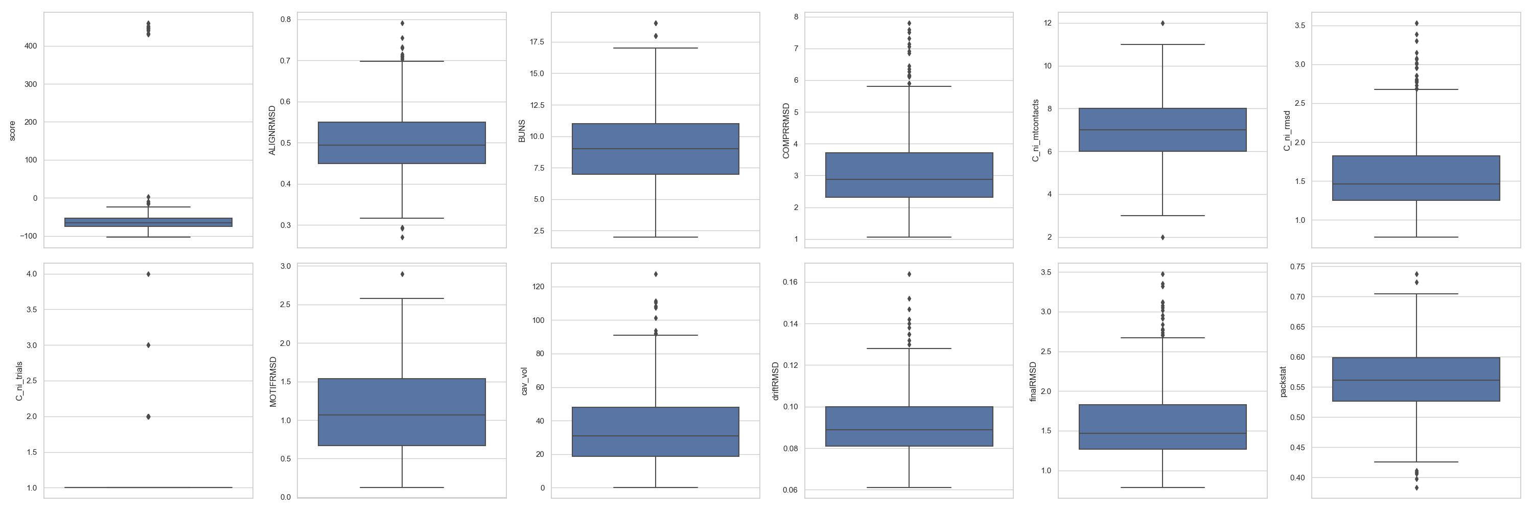
Tip

For multiple_distributions(), the grid has to define enough positions for all the scores expected to be plotted. In this case, there are 12 numerical columns and thus, that is the minimum number of cells necessary to plot.

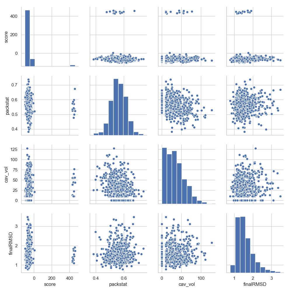
The structure of the DesignFrame is such that all one vs. one scores can directly be seen just be providing it to seaborn (let’s just select some scores to minimize the final image):

In [6]: grid = sns.pairplot(df[['score', 'packstat', 'cav_vol', 'finalRMSD']])

In [7]: plt.show()

Note

As a general rule, anything that a DataFrame can do, a DesignFrame also can.

Sorting and Selecting¶

One key part of the analysis of protein design datasets is the correct preselection of those designs potentially interesting. A DesignFrame can operate with all the same functions for sorting/selection that a DataFrame can.

Let’s make two populations: df_cr representing the top 10 scored decoys with a cav_vol <= 10 and a finalRMSD <= 1.5 and df_sr with the top 10 scored decoys with a packstat >= 0.6 and a finalRMSD <= 1.5.

In [8]: df_cr = df[(df['cav_vol'] <= 10) & (df['finalRMSD'] <= 1.5)].sort_values('score').head(10)
   ...: df_sr = df[(df['packstat'] >= 0.6) & (df['finalRMSD'] <= 1.5)].sort_values('score').head(10)
   ...: 

As can be seen in this example, selections can be concatenated with either & (AND - meaning that all conditions must be fulfilled) or | (OR - meaning that any of the conditions need to be met). After that, one can check the overlap between the two selected groups, either by checking the common identifiers as sets:

In [9]: print(set(df_cr['description'].values).intersection(df_sr['description'].values))
{'nubinitio_wauto_18326_2pw9C_0191_0001', 'nubinitio_wauto_18326_2pw9C_0147_0001'}

Or by merging only the common decoys, which will bring the full data:

In [10]: df_cr_sr = df_cr.merge(df_sr, how='inner', on='description', suffixes=['', '_2x'])

There are multiple options on how this two populations can be compared, if that might be needed to decide which is the one with a higher chance of success. Some of them are showcased in their specific tutorial.

Identification of Mutants¶

Identifying the mutations present in a population can be key to understand the sequence signatures behind the designs. It might be also a good starting point for new sets of designs as is explained in Generation of New Variants. Data referring to the identity and similarity with a reference_sequence is can easily be obtained by simple request (we will hide columns not currently informative for this example):

In [11]: df_sr = df_sr.identify_mutants('C')

Tip

Notice that the mutations are displayed on a basic sequence count; that is, assuming the protein sequence starts in 1. This is informative to keep on working on it, as numerical selection is performed that way, but to make a report the actual position might be more useful to get the count in the same range as the reference structure. One could get that format with report().

In [12]: rs.utils.report(df_sr[['description']].head(2))
Out[12]: 
                               description
209  nubinitio_wauto_18326_2pw9C_0213_0001
143  nubinitio_wauto_18326_2pw9C_0147_0001

Thanks to this quick identification, it is easy to select decoys with a particular sequence signature of interest through DesignFrame.get_sequence_with().

In [13]: df_sr.get_sequence_with('C', ((3, 'W'), (9, 'R')))
Out[13]: 
       score  ALIGNRMSD  BUNS  COMPRRMSD  C_ni_mtcontacts  C_ni_rmsd  C_ni_trials  MOTIFRMSD  cav_vol  driftRMSD  finalRMSD  packstat C_ni_rmsd_type                            description lbl_MOTIF lbl_SSE03 lbl_SSE05                                                  sequence_C                                                                                                                                                                                                                 mutants_C                                                                                                              mutant_positions_C  mutant_count_C
209 -102.402  0.533      8.0   1.931      8.0              1.222      1.0          1.656      10.279   0.094      1.274      0.618     no_motif       nubinitio_wauto_18326_2pw9C_0213_0001  [C]       [C]       [C]       SFWVIIRFRGVIVTIIDIDEPGELERAKEMLLRKGYLKKAEEGETAFFLPKGIAVISA  E1S,T2F,P3W,Y4V,A5I,A7R,L8F,N9R,D10G,R11V,V12I,I13V,G14T,S15I,S16I,M17D,V18I,L19D,P20E,V21P,D22G,L23E,E24L,F26R,G27A,A28K,G29E,F30M,F32L,G33R,Q34K,I37L,I43G,R44E,E45T,I46A,L47F,V48F,C49L,Q51K,R53I,I54A,S55V,V56I,Y57S  1,2,3,4,5,7,8,9,10,11,12,13,14,15,16,17,18,19,20,21,22,23,24,26,27,28,29,30,32,33,34,37,43,44,45,46,47,48,49,51,53,54,55,56,57  45            

One important issue when selecting which decoys will move to the next round or be selected for experimental validation is the sequence distance between them, to avoid (unless wanted) trying too similar designs:

In [14]: df_inner = df_sr.sequence_distance('C')

Or even to compare the sequences between two different selection criteria:

In [15]: df_outer = df_sr.sequence_distance('C', df_cr)

In [16]: fig = plt.figure(figsize=(30, 10))

In [17]: plt.show()

Visual Analysis of Mutations¶

Amino acid variation over all the decoys can be visualised in a variety of ways, always with the ability to select only regions of interest:

Through a sequence_frequency_plot():

In [18]: fig = plt.figure(figsize=(30, 10))

In [19]: plt.show()

As a logo_plot() (let’s see here only for the labeled region SSE03):

In [20]: sse03 = df_cr.get_label('SSE03', 'C').values[0]

In [21]: plt.show()

As a positional_sequence_similarity() (defaults to BLOSUM62 similarity matrix):

In [22]: fig  = plt.figure(figsize=(30, 10))

In [23]: plt.show()

And, finally, as an alignment with plot_alignment():

In [24]: fig  = plt.figure(figsize=(30, 10))

In [25]: plt.show()

Finally, a single selected decoy can be plotted individually with per_residue_matrix_score_plot(); in this case we will highlight the MOTIF region of interest and SSE05:

In [26]: fig  = plt.figure(figsize=(30, 10))

In [27]: plt.show()

In [28]: plt.close('all')