Generation of New Variants
A first round of designs might just be the stepping stone towards a second generation. It can be used to learn and better stir the next generation according to whatever is our final aim.
Note
All the examples here will generate new sequences. Once those new sequences are generated, we can generate with a call to DesignFrame.make_resfile()
the residue files that can be provided to Rosetta through the
ReadResfile to guide
the design process.
We are not calling the method in this tutorial as it generates files which cannot be shown.
Loading a Reference
As in Sequence Analysis, we will need to load a reference with get_sequence_and_structure().
Note
Through all the process several times the chainID of the decoy of interest will be called. This is due to the fact that the library can manipulate
decoys with multiple chains (designed or not), and, thus, analysis must be called upon the sequences of interest.
In [1]: import rstoolbox as rs
   ...: import pandas as pd
   ...: import matplotlib.pyplot as plt
   ...: import seaborn as sns
   ...: pd.set_option('display.width', 1000)
   ...: pd.set_option('display.max_columns', 500)
   ...: pd.set_option("display.max_seq_items", 3)
   ...: baseline = rs.io.get_sequence_and_structure('../rstoolbox/tests/data/2pw9C.pdb')
   ...: baseline.get_sequence('C')
   ...: baseline.add_reference_sequence('C', baseline.get_sequence('C'))
   ...: baseline.add_reference_shift('C', 32)
   ...:
Loading the Design Data
Again, we are mimicking Sequence Analysis.
In [2]: rules = {'scores_ignore': ['fa_*', 'niccd_*', 'hbond_*', 'lk_ball_wtd', 'pro_close', 'dslf_fa13', 'C_ni_rmsd_threshold',
   ...:                            'omega', 'p_aa_pp', 'yhh_planarity', 'ref', 'rama_prepro', 'time'],
   ...:          'sequence': 'C',
   ...:          'labels': ['MOTIF', 'SSE03', 'SSE05']}
   ...: df = rs.io.parse_rosetta_file('../rstoolbox/tests/data/input_ssebig.minisilent.gz', rules)
   ...: df.add_reference_sequence('C', baseline.get_sequence('C'))
   ...: df.add_reference_shift('C', 32)
   ...: df.head(3)
   ...:
Out[2]:
    score  ALIGNRMSD  BUNS  COMPRRMSD  C_ni_mtcontacts  C_ni_rmsd  C_ni_trials  MOTIFRMSD  cav_vol  driftRMSD  finalRMSD  packstat C_ni_rmsd_type                            description lbl_MOTIF lbl_SSE03 lbl_SSE05                                                  sequence_C
0 -64.070  0.608      12.0  7.585      4.0              3.301      1.0          0.957      66.602   0.083      3.323      0.544     no_motif       nubinitio_wauto_18326_2pw9C_0001_0001  [C]       [C]       [C]       TTWIKFFAGGTLVEEFEYSSVNWEEIEKRAWKKLGRWKKAEEGDLMIVYPDGKVVSWA
1 -70.981  0.639      12.0  2.410      8.0              1.423      1.0          0.737      0.000    0.094      1.395      0.552     no_motif       nubinitio_wauto_18326_2pw9C_0002_0001  [C]       [C]       [C]       NTWSTNILNGHPKITLLVEERGAEEIHLEWLKKQGLRKKAEENVYTTKLPNGAVKVYG
2 -43.863  0.480      8.0   4.279      6.0              2.110      1.0          0.819      93.641   0.110      2.106      0.575     no_motif       nubinitio_wauto_18326_2pw9C_0003_0001  [C]       [C]       [C]       PRWFIAMGDGVIWEIVLGSEQNLEEIAKKGLKRRGLYKKAEESIYTIIYPDGIAHTFG
Minimal Mutant
We’ve seen multiple ways to identify and view mutations in Sequence Analysis. Let’s imagine that we have identified a good decoy candidate but we want to try all the putative back mutations available. Basically, we ask if a less mutated decoy will perform as well as the one found.
For this, we will take the best scored decoy and we will try to generate_wt_reversions() on the residues belonging to strand 3 (SSE03) and 5 (SSE05):
In [3]: kres = df.get_label('SSE03', 'C').values[0] + df.get_label('SSE05', 'C').values[0]
...: ds = df.sort_values('score').iloc[0].generate_wt_reversions('C', kres)
...: ds.shape[0]
...:
Out[3]: 16384
In [4]: ds.head(4)
��������������Out[4]:
sequence_C description mutants_C mutant_positions_C mutant_count_C
0 SFWVIIRFRGVIVTIIDIDEPGELERAKEMLLRKGYLKKAEEGETAFFLPKGIAVISA nubinitio_wauto_18326_2pw9C_0213_0001 E1S,T2F,P3W,Y4V,A5I,A7R,L8F,N9R,D10G,R11V,V12I,I13V,G14T,S15I,S16I,M17D,V18I,L19D,P20E,V21P,D22G,L23E,E24L,F26R,G27A,A28K,G29E,F30M,F32L,G33R,Q34K,I37L,I43G,R44E,E45T,I46A,L47F,V48F,C49L,Q51K,R53I,I54A,S55V,V56I,Y57S 1,2,3,4,5,7,8,9,10,11,12,13,14,15,16,17,18,19,20,21,22,23,24,26,27,28,29,30,32,33,34,37,43,44,45,46,47,48,49,51,53,54,55,56,57 45
1 SFWVIIRFRGVIVTIIDIDEPGLEEFGAGFLFGKGYLKKAEEGETAFFLPKGRISVYA nubinitio_wauto_18326_2pw9C_0213_0001_v0001 E1S,T2F,P3W,Y4V,A5I,A7R,L8F,N9R,D10G,R11V,V12I,I13V,G14T,S15I,S16I,M17D,V18I,L19D,P20E,V21P,D22G,Q34K,I37L,I43G,R44E,E45T,I46A,L47F,V48F,C49L,Q51K 1,2,3,4,5,7,8,9,10,11,12,13,14,15,16,17,18,19,20,21,22,34,37,43,44,45,46,47,48,49,51 31
2 SFWVIIRFRGVIVTIIDIDEPGLEEFGAGFLFGKGYLKKAEEGETAFFLPKGRISVSA nubinitio_wauto_18326_2pw9C_0213_0001_v0002 E1S,T2F,P3W,Y4V,A5I,A7R,L8F,N9R,D10G,R11V,V12I,I13V,G14T,S15I,S16I,M17D,V18I,L19D,P20E,V21P,D22G,Q34K,I37L,I43G,R44E,E45T,I46A,L47F,V48F,C49L,Q51K,Y57S 1,2,3,4,5,7,8,9,10,11,12,13,14,15,16,17,18,19,20,21,22,34,37,43,44,45,46,47,48,49,51,57 32
3 SFWVIIRFRGVIVTIIDIDEPGLEEFGAGFLFGKGYLKKAEEGETAFFLPKGRISIYA nubinitio_wauto_18326_2pw9C_0213_0001_v0003 E1S,T2F,P3W,Y4V,A5I,A7R,L8F,N9R,D10G,R11V,V12I,I13V,G14T,S15I,S16I,M17D,V18I,L19D,P20E,V21P,D22G,Q34K,I37L,I43G,R44E,E45T,I46A,L47F,V48F,C49L,Q51K,V56I 1,2,3,4,5,7,8,9,10,11,12,13,14,15,16,17,18,19,20,21,22,34,37,43,44,45,46,47,48,49,51,56 32
Note
To avoid confusion, all scores are unattached from the sequences, as they will need to be recalculated.
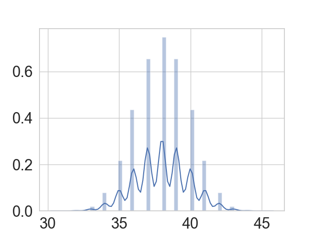
Mind that this will create all the combinatorial options from the selected mutant to the original wild type for the selected residues.
In [5]: _ = sns.distplot(ds['mutant_count_C'].values)

In [6]: plt.show()
Defining New Mutations of Interest
Let’s say that, after inspecting scores and visualising structures, there are some key positions for which seems relevant to try some particular residue types, that can also be controlled (also,
remember form Sequence Analysis that we can select already decoys with some particular mutations with DesignFrame.get_sequence_with()). This functionality comes by the
hand of DesignFrame.generate_mutant_variants(). Let’s now try it for the two best scored decoys.
In [7]: mutants = [(20, "AIV"), (31, "EDQR")]
...: ds = df.sort_values('score').iloc[:2].generate_mutant_variants('C', mutants)
...: ds.shape[0]
...:
Out[7]: 26
In [8]: ds.head(4)
�����������Out[8]:
sequence_C description mutants_C mutant_positions_C mutant_count_C
0 SFWVIIRFRGVIVTIIDIDEPGELERAKEMLLRKGYLKKAEEGETAFFLPKGIAVISA nubinitio_wauto_18326_2pw9C_0213_0001 E1S,T2F,P3W,Y4V,A5I,A7R,L8F,N9R,D10G,R11V,V12I,I13V,G14T,S15I,S16I,M17D,V18I,L19D,P20E,V21P,D22G,L23E,E24L,F26R,G27A,A28K,G29E,F30M,F32L,G33R,Q34K,I37L,I43G,R44E,E45T,I46A,L47F,V48F,C49L,Q51K,R53I,I54A,S55V,V56I,Y57S 1,2,3,4,5,7,8,9,10,11,12,13,14,15,16,17,18,19,20,21,22,23,24,26,27,28,29,30,32,33,34,37,43,44,45,46,47,48,49,51,53,54,55,56,57 45
1 SFWVIIRFRGVIVTIIDIDAPGELERAKEMELRKGYLKKAEEGETAFFLPKGIAVISA nubinitio_wauto_18326_2pw9C_0213_0001_v0001 E1S,T2F,P3W,Y4V,A5I,A7R,L8F,N9R,D10G,R11V,V12I,I13V,G14T,S15I,S16I,M17D,V18I,L19D,P20A,V21P,D22G,L23E,E24L,F26R,G27A,A28K,G29E,F30M,L31E,F32L,G33R,Q34K,I37L,I43G,R44E,E45T,I46A,L47F,V48F,C49L,Q51K,R53I,I54A,S55V,V56I,Y57S 1,2,3,4,5,7,8,9,10,11,12,13,14,15,16,17,18,19,20,21,22,23,24,26,27,28,29,30,31,32,33,34,37,43,44,45,46,47,48,49,51,53,54,55,56,57 46
2 SFWVIIRFRGVIVTIIDIDAPGELERAKEMDLRKGYLKKAEEGETAFFLPKGIAVISA nubinitio_wauto_18326_2pw9C_0213_0001_v0002 E1S,T2F,P3W,Y4V,A5I,A7R,L8F,N9R,D10G,R11V,V12I,I13V,G14T,S15I,S16I,M17D,V18I,L19D,P20A,V21P,D22G,L23E,E24L,F26R,G27A,A28K,G29E,F30M,L31D,F32L,G33R,Q34K,I37L,I43G,R44E,E45T,I46A,L47F,V48F,C49L,Q51K,R53I,I54A,S55V,V56I,Y57S 1,2,3,4,5,7,8,9,10,11,12,13,14,15,16,17,18,19,20,21,22,23,24,26,27,28,29,30,31,32,33,34,37,43,44,45,46,47,48,49,51,53,54,55,56,57 46
3 SFWVIIRFRGVIVTIIDIDAPGELERAKEMQLRKGYLKKAEEGETAFFLPKGIAVISA nubinitio_wauto_18326_2pw9C_0213_0001_v0003 E1S,T2F,P3W,Y4V,A5I,A7R,L8F,N9R,D10G,R11V,V12I,I13V,G14T,S15I,S16I,M17D,V18I,L19D,P20A,V21P,D22G,L23E,E24L,F26R,G27A,A28K,G29E,F30M,L31Q,F32L,G33R,Q34K,I37L,I43G,R44E,E45T,I46A,L47F,V48F,C49L,Q51K,R53I,I54A,S55V,V56I,Y57S 1,2,3,4,5,7,8,9,10,11,12,13,14,15,16,17,18,19,20,21,22,23,24,26,27,28,29,30,31,32,33,34,37,43,44,45,46,47,48,49,51,53,54,55,56,57 46
Exhaustive Point Mutant Sampling
An interesting approach could also be to create the appropriate data to exhaustively explore all possible point mutant in all possible
positions. This is extremely easy to do with the rstoolbox, generating a total of (len(sequence) * 19) + 1 variants:
In [9]: point_mutants = []
   ...: for i in range(1, len(baseline.get_reference_sequence('C')) + 1):
   ...:     mutation = [(i, "*")]
   ...:     point_mutants.append(baseline.generate_mutant_variants('C', mutation))
   ...: point_mutants = pd.concat(point_mutants).drop_duplicates('sequence_C')
   ...: print(','.join(point_mutants['mutants_C'].sample(frac=0.035)))  # show only some...
   ...:
A58Y,G14E,V56L,A5I,V18L,R11V,M17A,E1Y,L8T,P3S,V21G,I6N,A5H,S16Y,E41R,E41W,A28H,D10R,M17W,L31R,R44L,N9I,L31W,E41M,L47A,A40P,F30Q,F26D,N9P,A40M,R11W,I13Y,G33S,E1Q,F26M,I6L,V21K,N9C,A58N
With small variations, this same loop can be used to generate this exhaustive scanning over particular residues or to only scan specific residue types (for example to perform an Alanine Scanning).
Learning from Amino Acids Frequency
Instead of manually checking the positions and residue types of interest, one could learn from different sources to improve the type of sequences that one could get.
This new decoy sequences will be scored according to the frequency matrix they were generated from, but any decoy can be mapped to a sequence matrix with
DesignFrame.score_by_pssm().
For instance, one could get the information content of the 15 top scored decoys and try to obtain a certain amount of mutants (10) from the two best packed decoy that would
actually follow the statistical rules of that set with DesignFrame.generate_mutants_from_matrix():
In [10]: df15 = df.sort_values('score').iloc[:15].sequence_frequencies('C')
   ....: df.sort_values('packstat', ascending=False).iloc[:2].generate_mutants_from_matrix('C', df15, 10)
   ....:
Out[10]:
[                                   description                                                  sequence_C  pssm_score_C
 0  nubinitio_wauto_18326_2pw9C_0260_0001_v0001  RTPVEVKFNGELVTMLDSNGRRQKEIAYAELLKQGLWKKAEEGKYTIIYPDGWVVFVG  23.200000
 1  nubinitio_wauto_18326_2pw9C_0260_0001_v0002  PTVVVVRLGGQPISRQLRDLINLEEIAKEFMRKLGYAKKAEEGQKVVIEPDGSIISAD  24.866667
 2  nubinitio_wauto_18326_2pw9C_0260_0001_v0003  KKWLVVMLRGVPKIVIYVLNSNLEEEAREYLREQGLWKKAEEGTYTIVYSKGYIRTSA  23.933333
 3  nubinitio_wauto_18326_2pw9C_0260_0001_v0004  GQWIYVMFRGVPIKVMDIKDKNEEEEAWEMLKKKGVWKKAEEGKYVYILPNGYVITAA  24.733333
 4  nubinitio_wauto_18326_2pw9C_0260_0001_v0005  LFWVEFFFNGVPTFMLLSEDIGEEEIARRIFKKKGLLKKAEEGTYVMYLPDGIVEISD  25.666667
 5  nubinitio_wauto_18326_2pw9C_0260_0001_v0006  NTWVLVRFRGVPKTVLLTNNRGQLEIAREEMRKLGLMKKAEEDIYIRFLPNGIVIISP  24.400000
 6  nubinitio_wauto_18326_2pw9C_0260_0001_v0007  PFWVVVELNGVPIIVQIVVPIGEEEIAREYQKKQGVWKKAEEGQEGEYYPDGVLLIYG  25.333333
 7  nubinitio_wauto_18326_2pw9C_0260_0001_v0008  PQVFVFETGGEPKTIQIINDKNQEELAEKEYKRLGQGKKAEEGKTVMIYPNGVIYFYG  23.266667
 8  nubinitio_wauto_18326_2pw9C_0260_0001_v0009  PTWVEFFFNGEPIMILLTTGSGLKERAWEYLKKMGQLKKAEEGEYVVFSPNGWIEHYA  24.866667
 9  nubinitio_wauto_18326_2pw9C_0260_0001_v0010  PQWLVFEVNGVLKTMQLRVNPNLLEIAYRLLRKLGLWKKAEEGTETIILSDGIVLSSE  24.000000   ,
                                    description                                                  sequence_C  pssm_score_C
 0  nubinitio_wauto_18326_2pw9C_0278_0001_v0001  KKVFEVRYNGVPTSVLLTNNTGLEEIALRLLKRQGQWKKAEEGEFSIIYPNGAVIFYP  24.666667
 1  nubinitio_wauto_18326_2pw9C_0278_0001_v0002  TTLIKFMLNGVPVTMQLSEGSNLLEYAYKLQKKQGLLKKAEEGKTVYIYSKGEVRFWA  23.733333
 2  nubinitio_wauto_18326_2pw9C_0278_0001_v0003  PTWVVFFTNGVPKSRILTEDSNLEEIGEREMKKLGVWKKAEEGKYVIVKPDGIVIIVG  26.466667
 3  nubinitio_wauto_18326_2pw9C_0278_0001_v0004  KTWVEVRFNGEPITISLLNGRNIEEAAYRELKKKGLLKKAEEGKEVEVYPSGIILHAA  26.866667
 4  nubinitio_wauto_18326_2pw9C_0278_0001_v0005  GIWVVIRVNGEPISVLATKGKNLEEIAREEFRKLGLMKKAEENKYVEEYPKGVIWIYD  25.533333
 5  nubinitio_wauto_18326_2pw9C_0278_0001_v0006  TFWVEVKLNGVPKIVMLVENINEKEIAREELKKMGLLKKAEESKYVRIYPDGVVYTFG  26.866667
 6  nubinitio_wauto_18326_2pw9C_0278_0001_v0007  LTPFVIRVNGQPITMILVVNSNEEERAREELKRKGLLKKAEEGKFVYFEPKGVAYSYG  25.466667
 7  nubinitio_wauto_18326_2pw9C_0278_0001_v0008  STWVYFRVNGEPISVVLVNNRNQEERARREQRRKGLWKKAEESEEVIIYSDGVVYSTG  24.933333
 8  nubinitio_wauto_18326_2pw9C_0278_0001_v0009  SQWVVVRVRGVPIKRILVTPKNQEEIAYEELKKQGKWKKAEEGTTAIILPKGEIWFYD  25.933333
 9  nubinitio_wauto_18326_2pw9C_0278_0001_v0010  PIPVEVKFNGVPIKMIAIVDIKEEKYAREFLKKQGLAKKAEEDKTVIFLPDGELWSYA  23.866667   ]
Note
While the generation of the best scored sequence according to a matrix is quite straight forward, the generation of the N best is not. Thus, the way a frequency matrix is applied in this scenario is that the frequency corrects a randomised selection per position. Statistically, this will make most sequences obtained on the upper side of the matrix score.
Creating the New Mutants
After generating new variations, those can be run in Rosetta to obtain their corresponding scores with DesignFrame.apply_resfile. By default, this function will run
fixed backbone design with a script such as:
In [11]: print(rs.utils.mutations())
<ROSETTASCRIPTS>
    <TASKOPERATIONS>
        <ReadResfile name="targets" filename="%%resfile%%"/>
    </TASKOPERATIONS>
    <MOVERS>
        <PackRotamersMover name="packrot" task_operations="targets" />
        <AddJobPairData name="annotate" value_type="string"
                        key="resfile_A" value="%%resfile%%" />
    </MOVERS>
    <PROTOCOLS>
        <Add mover="packrot" />
        <Add mover="annotate" />
    </PROTOCOLS>
</ROSETTASCRIPTS>
But the user can provide more complex RosettaScripts to execute, as long as they follow the same restrictions as this one:
- They contain the AddJobPairData Mover.
- They target the resfile with the
script_var%%resfile%%.