Compare Decoy Populations
Comparing features between populations is one of the best ways to benchmark different conditions in an experiment.
This example works over two populations designed in the same manner, with the only difference that one was performed in the presence of a binder while the other was design alone.
We are ignoring some scores to facilitate general reading, but this particularity is not mentioned any more during the tutorial. Similarly, we are using only a sample of the 20K available sequences on each decoy population.
In [1]: import rstoolbox as rs
...: import pandas as pd
...: import numpy as np
...: pd.set_option('display.width', 1000)
...: pd.set_option('display.max_columns', 500)
...: pd.set_option("display.max_seq_items", 3)
...: binder = rs.io.parse_rosetta_file('../rstoolbox/tests/data/compare/binder.mini.gz', {'sequence': 'B', 'scores_ignore': ['time', 'fa_*', 'dslf_fa13', 'yhh_planarity', 'pro_close']}).sample(frac=0.05)
...: binder.columns.values
...:
Out[1]:
array(['score', 'hbond_sr_bb', 'hbond_lr_bb', 'hbond_bb_sc', 'hbond_sc',
'rama', 'omega', 'p_aa_pp', 'ref', 'BUNS', 'B_ni_mtcontacts',
'B_ni_rmsd', 'B_ni_rmsd_threshold', 'B_ni_trials', 'GRMSD2Target',
'GRMSD2Template', 'LRMSD2Target', 'LRMSDH2Target',
'LRMSDLH2Target', 'cav_vol', 'design_score', 'packstat',
'rmsd_drift', 'description', 'sequence_B'], dtype=object)
In [2]: nobinder = rs.io.parse_rosetta_file('../rstoolbox/tests/data/compare/nobinder.mini.gz', {'sequence': 'B', 'scores_ignore': ['time', 'fa_*', 'dslf_fa13', 'yhh_planarity', 'pro_close']}).sample(frac=0.05)
...: nobinder.columns.values
...:
����������������������������������������������������������������������������������������������������������������������������������������������������������������������������������������������������������������������������������������������������������������������������������������������������������������������������������������������������������������������������������������������������������������������������Out[2]:
array(['score', 'hbond_sr_bb', 'hbond_lr_bb', 'hbond_bb_sc', 'hbond_sc',
'rama', 'omega', 'p_aa_pp', 'ref', 'BUNS', 'B_ni_mtcontacts',
'B_ni_rmsd', 'B_ni_rmsd_threshold', 'B_ni_trials', 'GRMSD2Target',
'GRMSD2Template', 'LRMSD2Target', 'LRMSDH2Target',
'LRMSDLH2Target', 'cav_vol', 'design_score', 'packstat',
'rmsd_drift', 'description', 'sequence_B'], dtype=object)
Merging Populations
Merging populations is a very useful way to a take advantage of the plotting and analysis tools compatible with DataFrame derived objects. In order
for it to be useful and possible, two conditions must meet:
There must be a column to identify to which population each decoy belongs
In this example, none exist. But if we take a look at the naming of the decoys:
In [4]: print("{0} <-> {1}".format(binder.iloc[0]['description'], nobinder.iloc[0]['description']))
classicFFL_FFL_binder_motif_DesignRelax_noaa_pack_13636_3lhp_0196 <-> classicFFL_FFL_nobinder_motif_DesignRelax_noaa_30229_3lhp_0002
We could see that, by loading the data not with the definition {'sequence': 'B'} but with {'sequence': 'B', 'naming': ['', '', 'condition']} we would
have automatically obtained a column condition defining the binder presence.
As we did not do that, or in case that would not be possible, we will just add an extra column.
In [5]: binder = rs.utils.add_column(binder, 'condition', 'binder')
...: binder.columns.values
...:
Out[5]:
array(['score', 'hbond_sr_bb', 'hbond_lr_bb', 'hbond_bb_sc', 'hbond_sc',
'rama', 'omega', 'p_aa_pp', 'ref', 'BUNS', 'B_ni_mtcontacts',
'B_ni_rmsd', 'B_ni_rmsd_threshold', 'B_ni_trials', 'GRMSD2Target',
'GRMSD2Template', 'LRMSD2Target', 'LRMSDH2Target',
'LRMSDLH2Target', 'cav_vol', 'design_score', 'packstat',
'rmsd_drift', 'description', 'sequence_B', 'condition'],
dtype=object)
In [6]: nobinder = rs.utils.add_column(nobinder, 'condition', 'nobinder')
...: nobinder.columns.values
...:
�����������������������������������������������������������������������������������������������������������������������������������������������������������������������������������������������������������������������������������������������������������������������������������������������������������������������������������������������������������������������������������������������������������������������������������������������Out[6]:
array(['score', 'hbond_sr_bb', 'hbond_lr_bb', 'hbond_bb_sc', 'hbond_sc',
'rama', 'omega', 'p_aa_pp', 'ref', 'BUNS', 'B_ni_mtcontacts',
'B_ni_rmsd', 'B_ni_rmsd_threshold', 'B_ni_trials', 'GRMSD2Target',
'GRMSD2Template', 'LRMSD2Target', 'LRMSDH2Target',
'LRMSDLH2Target', 'cav_vol', 'design_score', 'packstat',
'rmsd_drift', 'description', 'sequence_B', 'condition'],
dtype=object)
Once all conditions are met, the populations can be merged:
In [7]: df = pd.concat([binder, nobinder], ignore_index=True)
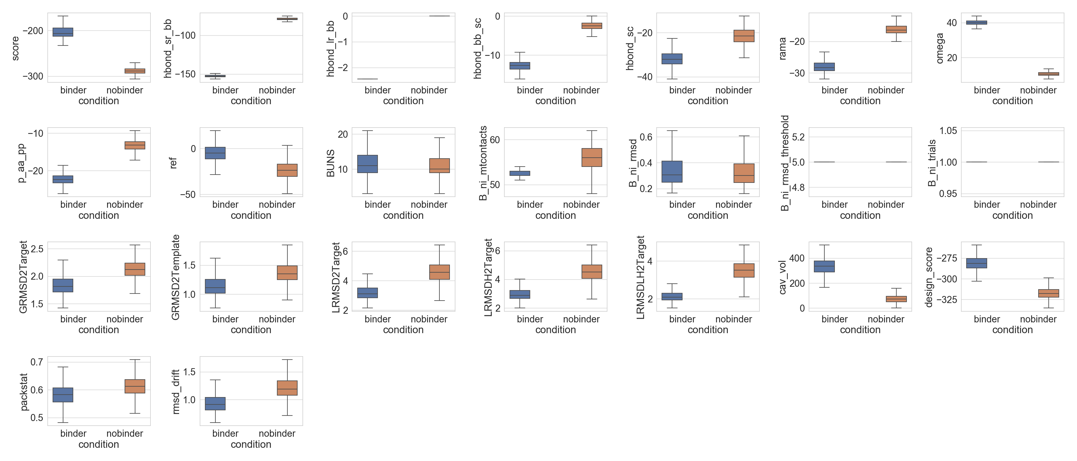
Comparing Basic Scores
The first and most straight forward analysis between populations is the comparison between their different scores distributions. For that,
multiple_distributions() accepts any attribute of boxplot(), so that data can be properly separated.
In [8]: import matplotlib.pyplot as plt
   ...: import seaborn as sns
   ...: fig  = plt.figure(figsize=(35, 15))
   ...: grid = [4, 7]
   ...: axes = rs.plot.multiple_distributions( df, fig, grid, x='condition', hue='condition', showfliers=False )
   ...: nones = [x.legend_.remove() for x in axes]
   ...: plt.tight_layout()
   ...:

In [9]: plt.show()
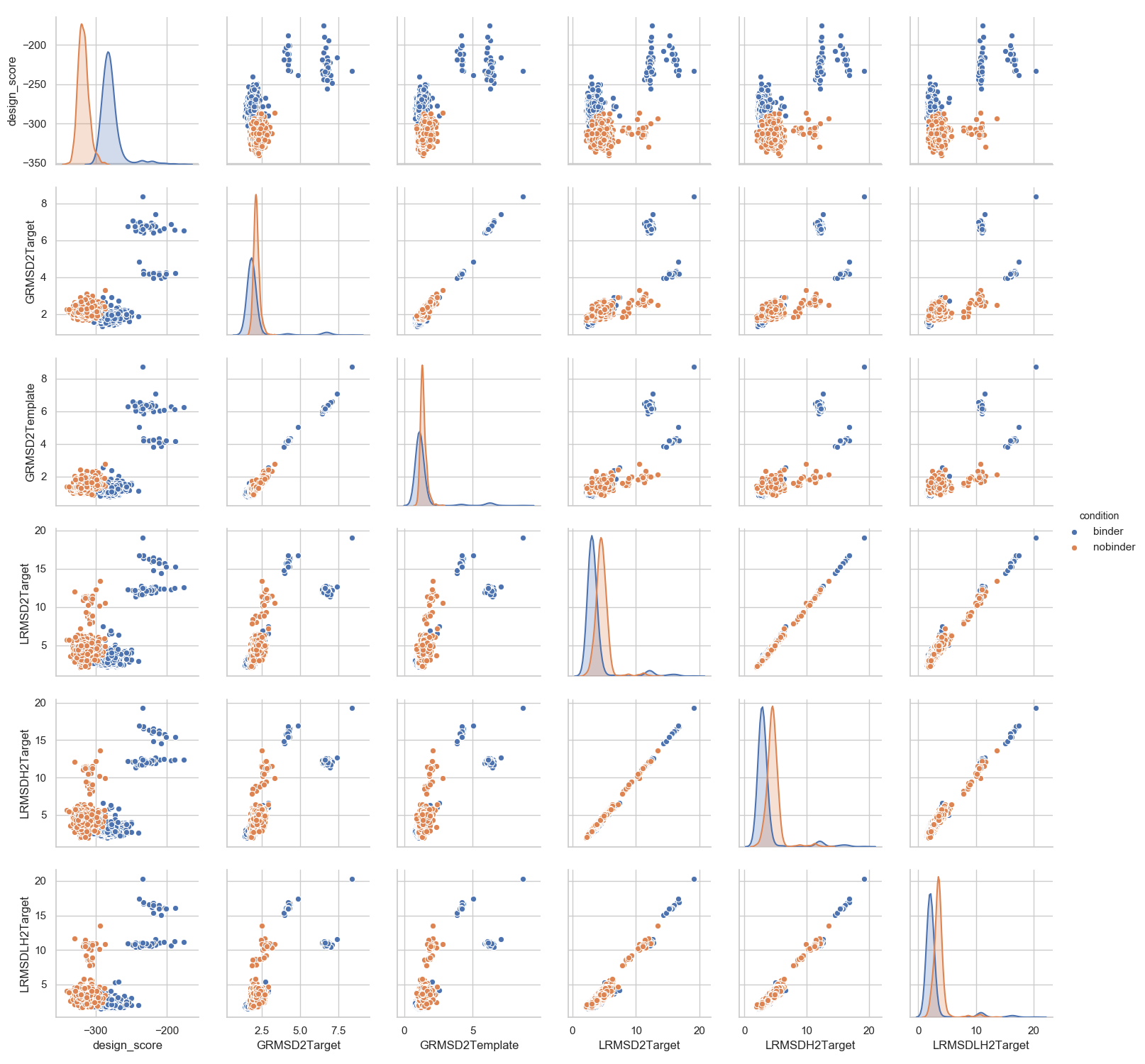
The data can even be directly used on seaborn functions:
In [10]: sns.set(font_scale=1)
   ....: sns.set_style("whitegrid")
   ....: _ = sns.pairplot(df[['design_score', 'GRMSD2Target', 'GRMSD2Template', 'LRMSD2Target', 'LRMSDH2Target', 'LRMSDLH2Target', 'condition']],
   ....:                  hue='condition')
   ....:

In [11]: plt.show()
More specific comparisons can be performed depending on the actual aim of the project.
Sequence Distances
Let’s assume that one wants to evaluate the spread of the two populations and how well they recover a given target reference sequence. For that, we will need to provide a reference sequence.
In [12]: reference = rs.io.get_sequence_and_structure('../rstoolbox/tests/data/compare/4oyd.pdb', {'sequence': 'B'})
   ....: _ = df.add_reference_sequence('B', reference.iloc[0].get_sequence('B')[:-1])
   ....:
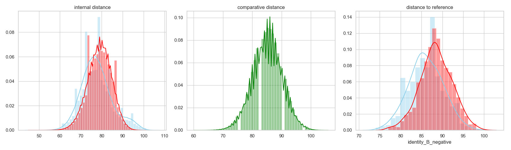
A tutorial for population sequence analysis is also available, but there are options that can be used when comparing two populations.
For instance, one can evaluate the internal sequence inside each decoy population and then compare it between the two:
In [13]: disbinder = df[df['condition'] == 'binder'].sequence_distance('B')
   ....: disbinder = disbinder.mask(np.triu(np.ones(disbinder.shape, dtype=np.bool_))) # mask diagonal and upper diagonal values
   ....: disbinder = disbinder.values.flatten() # to array
   ....: disbinder = disbinder[[~np.isnan(disbinder)]] # clean NaN
   ....:
   ....: disnobinder = df[df['condition'] == 'nobinder'].sequence_distance('B')
   ....: disnobinder = disnobinder.mask(np.triu(np.ones(disnobinder.shape, dtype=np.bool_))) # mask diagonal and upper diagonal values
   ....: disnobinder = disnobinder.values.flatten() # to array
   ....: disnobinder = disnobinder[[~np.isnan(disnobinder)]] # clean NaN
   ....:
Or evaluate the distance between the two sequence populations:
In [14]: discomp = df[df['condition'] == 'binder'].sequence_distance('B', df[df['condition'] == 'nobinder'])
   ....: discomp = discomp.values.flatten() # to array
   ....: discomp = discomp[[~np.isnan(discomp)]] # clean NaN
   ....:
Or the distance of each group to the reference sequence:
In [15]: disbinderref = rs.analysis.sequence_similarity(df[df['condition'] == 'binder'], 'B', matrix='IDENTITY')['identity_B_negative']
   ....: disnobinderref = rs.analysis.sequence_similarity(df[df['condition'] == 'nobinder'], 'B', matrix='IDENTITY')['identity_B_negative']
   ....:
We can show all this together as:
In [16]: fig  = plt.figure(figsize=(17, 5))
   ....: grid = [1, 3]
   ....: ax00 = plt.subplot2grid(grid, (0, 0))
   ....: _ = sns.distplot( disbinder , color="skyblue", label="binder", ax=ax00)
   ....: _ = sns.distplot( disnobinder , color="red", label="nobinder", ax=ax00)
   ....: rs.utils.add_top_title(ax00, 'internal distance')
   ....: ax01 = plt.subplot2grid(grid, (0, 1))
   ....: _ = sns.distplot( discomp , color="green", label="binder vs. nobinder", ax=ax01)
   ....: rs.utils.add_top_title(ax01, 'comparative distance')
   ....: ax02 = plt.subplot2grid(grid, (0, 2))
   ....: _ = sns.distplot( disbinderref , color="skyblue", label="binder", ax=ax02)
   ....: _ = sns.distplot( disnobinderref , color="red", label="nobinder", ax=ax02)
   ....: rs.utils.add_top_title(ax02, 'distance to reference')
   ....: plt.tight_layout()
   ....:

In [17]: plt.show()
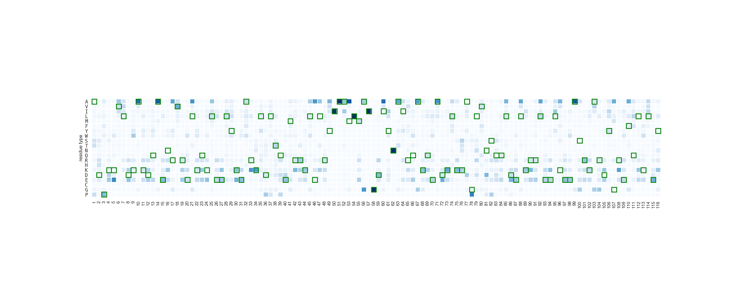
To fully asses the difference between the two populations, we can evaluate the enrichment of different residue types in different positions. In this scenario, we will measure the enrichment of variants in the binder-designed population against the other. This entails that high values represent residue types more present in the binder-design population per position.
In [18]: result = rs.analysis.positional_enrichment(df[df['condition'] == 'binder'], df[df['condition'] == 'nobinder'], 'B')
When a position is represented in the first population but not in the second, the enrichment is inf. To visualize it,
one would need to transform it into a numerical value. In this case, we transform it into a value such as max + (max/2).
In [19]: maxval = result.replace(np.inf, -1).max().max()
   ....: maxval += (maxval / float(2))
   ....: result = result.replace(np.inf, maxval)
   ....: fig = plt.figure(figsize=(25, 10))
   ....: ax = plt.subplot2grid((1, 1), (0, 0))
   ....: rs.plot.sequence_frequency_plot(df, "B", ax, cbar=False, xrotation=90)
   ....:

In [20]: plt.show()
Comparing enrichment between the populations (i.e. full sequence enrichment) is demonstrated in the experimental analysis tutorial.