Experimental Data
Experimental data derived from the analysis of the design decoys can be added and processed through the library. For some experiments, like
Circular Dichroism or Surface Plasmon Resonance, very specific formats exist. In those cases, the proper parser (read_CD() or
read_SPR()) exists. Other cases provide different +*CSV* files. This can be imported to python with read_csv(), but might
need to be post-processed to work with them.
Each plotting function shows in its documentation the exact naming of the column that it expects.
Circular Dichroism
Circular dichroism data can be easily worked with.
Currently the library can automatically import data compatible with the Jasco J-815
series by means of the read_CD() function, but any data can be read as long as it finally produces a DataFrame with, at least, the following
two columns:
| Column Name | Data Content |
|---|---|
| Wavelength | Wavelength (nm). |
| MRE | Value at each wavelength (10 deg^2 cm^2 dmol^-1). |
Adding a new available format to the library would be as easy as adding the appropriate private function to rstoolbox/io/experimental and provide access to
it through the read_CD() function.
Note
When loading data with read_CD() notice that the DataFrame contains extra columns with extra information. From those, Temp is the more relevant for
plotting and analysis, as is the one that allows to separate the different data series.
Currently, CD data can be obtained and plotted such as:
In [1]: import rstoolbox as rs
   ...: dfCD = rs.io.read_CD("../rstoolbox/tests/data/CD", model='J-815')
   ...: dfCD.columns
   ...:
Out[1]: Index(['Wavelength', 'MRE', 'voltage', 'title', 'bin', 'minw', 'Temp'], dtype='object')

In [2]: import matplotlib.pyplot as plt
   ...: fig = plt.figure(figsize=(10, 6.7))
   ...: ax = plt.subplot2grid((1, 1), (0, 0), fig=fig)
   ...: rs.plot.plot_CD(dfCD, ax, sample=6)
   ...:

In [3]: plt.show()
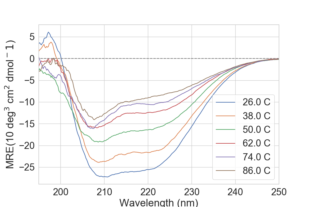
Tip
Depending on how many temperatures one might have, trying to plot all of them will create a very large legend. One can either delete it or use the sample option, which
uses the Bresenham’s line algorithm to sample temperatures across all possible
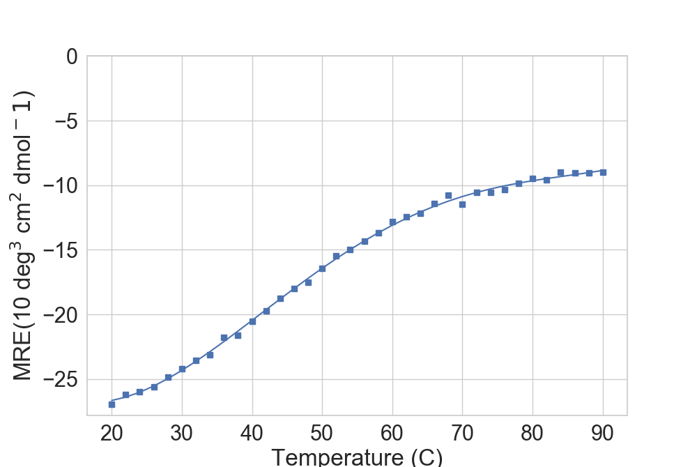
Thermal Melt
As before, thermal melt data can be loaded by properly parsing any input file as long as the generated DataFrame contains at least the following columns:
| Column Name | Data Content |
|---|---|
| Temp | Temperatures (celsius). |
| MRE | Value at each temperature (10 deg^2 cm^2 dmol^-1). |
If loaded from CD data containing a temp column (as is the case when loaded with read_CD()), one can directly pick the data from there:
In [4]: dfTM = dfCD[(dfCD['Wavelength'] == 220)]
   ...: fig = plt.figure(figsize=(10, 6.7))
   ...: ax = plt.subplot2grid((1, 1), (0, 0), fig=fig)
   ...: rs.plot.plot_thermal_melt(dfTM, ax)
   ...:

In [5]: plt.show()
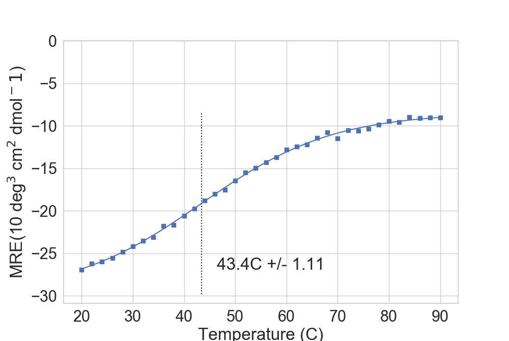
For well-behaved proteins, the library can approximate the melting point.
In [6]: fig = plt.figure(figsize=(10, 6.7))
   ...: ax = plt.subplot2grid((1, 1), (0, 0), fig=fig)
   ...: rs.plot.plot_thermal_melt(dfTM, ax, fusion_temperature=True, temp_marker=True)
   ...:

In [7]: plt.show()
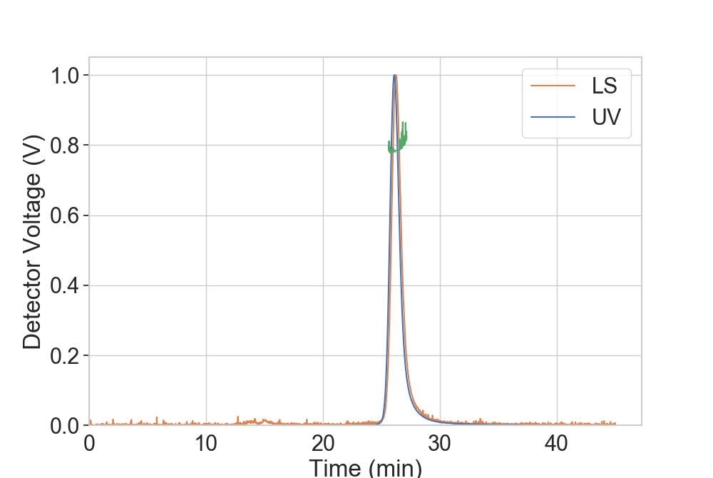
Multi-Angle Light Scattering
MALS data can be manually loaded or read through the read_MALS() function.
In order to properly work with the plotting functions, it needs to have at least two of the following columns:
| Column Name | Data Content |
|---|---|
| Time | Time (min). |
| UV | UV data (V). |
| LS | Light Scattering data (V). |
| MW | Molecular Weight (Daltons). |
being Time always mandatory. Depending on the amount of data, the plot function can pick which information to print.
In [8]: import pandas as pd
   ...: dfMALS = pd.read_csv("../rstoolbox/tests/data/mals.csv")
   ...: fig = plt.figure(figsize=(10, 6.7))
   ...: ax = plt.subplot2grid((1, 1), (0, 0))
   ...: rs.plot.plot_MALS(dfMALS, ax)
   ...:

In [9]: plt.show()
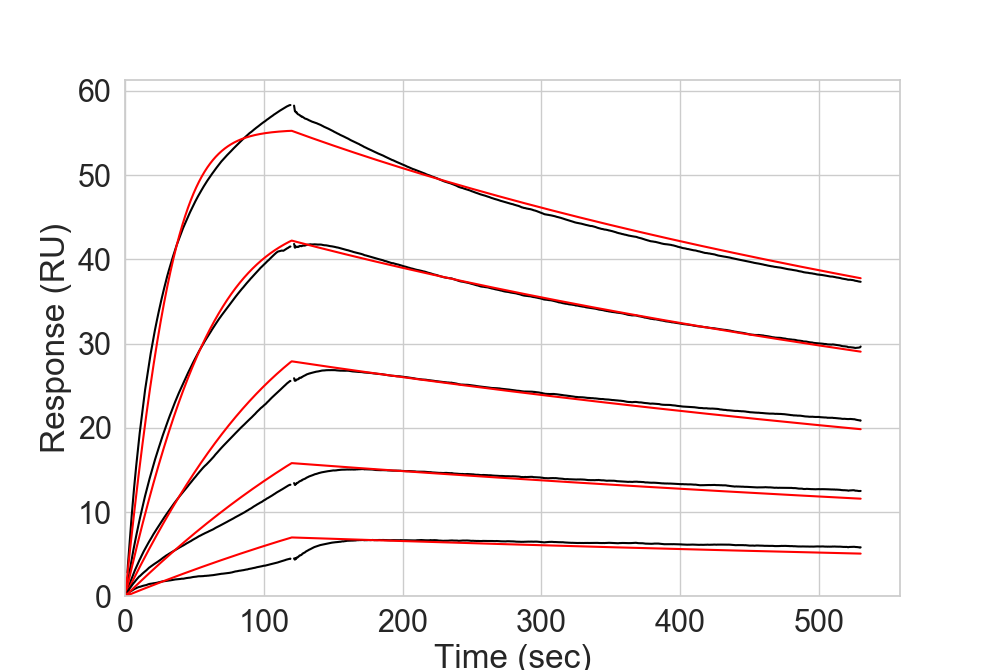
Surface Plasmon Resonance
Optimal SPR data has to contain the fitted curves on input, but can be read directly from the default output of the machine.
More details on the format are listed in the corresponding function read_SPR().
The fitted curves will be directly represented with plot_SPR().
In [10]: dfSPR = rs.io.read_SPR("../rstoolbox/tests/data/spr_data.csv.gz")
   ....: fig = plt.figure(figsize=(10, 6.7))
   ....: ax = plt.subplot2grid((1, 1), (0, 0))
   ....: rs.plot.plot_SPR(dfSPR, ax, datacolor='black', fitcolor='red')
   ....:

In [11]: plt.show()

In [12]: plt.close('all')
Deep Sequence Analysis and Population Enrichment
Individual raw FASTQ data obtained from deep sequencing can be directly read with the read_fastq() function.
In order to evaluate the enrichment of different outputs submitted to a different experimental conditions in different
concentrations, and provide the min and max concentrations to use for the calculus to sequence_enrichment().
In [13]: indat = {'binder1': {'conc1': '../rstoolbox/tests/data/cdk2_rand_001.fasq.gz',
   ....:                      'conc2': '../rstoolbox/tests/data/cdk2_rand_002.fasq.gz',
   ....:                      'conc3': '../rstoolbox/tests/data/cdk2_rand_003.fasq.gz'},
   ....:          'binder2': {'conc1': '../rstoolbox/tests/data/cdk2_rand_004.fasq.gz',
   ....:                      'conc2': '../rstoolbox/tests/data/cdk2_rand_005.fasq.gz',
   ....:                      'conc3': '../rstoolbox/tests/data/cdk2_rand_006.fasq.gz'}}
   ....: enrich = {'binder1': ['conc1', 'conc3'],
   ....:           'binder2': ['conc1', 'conc3']}
   ....: dfSeq = rs.utils.sequencing_enrichment(indat, enrich)
   ....: dfSeq[[_ for _ in dfSeq.columns if _ != 'sequence_A']].head()
   ....:
Out[13]:
   description  binder1_conc1  binder1_conc2  binder1_conc3  binder2_conc1  binder2_conc2  binder2_conc3  len  enrichment_binder1  enrichment_binder2
0  0            4.0            1.0            0.0            1.0            0.0            3.0            304 -1.00                0.333333
1  1            4.0            2.0            1.0            2.0            1.0            0.0            304  4.00               -1.000000
2  2            3.0            2.0            4.0            1.0            1.0            1.0            304  0.75                1.000000
3  3            3.0            1.0            1.0            1.0            0.0            3.0            304  3.00                0.333333
4  4            3.0            0.0            1.0            2.0            2.0            1.0            298  3.00                2.000000