rstoolbox.plot.multiple_distributions¶

rstoolbox.plot.multiple_distributions(df, fig, grid, igrid=None, values='*', titles=None, labels=None, refdata=None, ref_equivalences=None, violins=True, legends=False, **kwargs)¶

Automatically plot boxplot distributions for multiple score types of the decoy population.

A part from the fixed options, the function accepst any option of boxplot(), except for y, data and ax, which are used internally by this function.

Parameters:

df (DataFrame) – Data container.
fig (Figure) – Figure into which the data is going to be plotted.
grid (tuple with two int) – Shape of the grid to plot the values in the figure (rows x columns).
igrid (tuple with two int) – Initial position of the grid. Defaults to (0, 0)
values (list() of str) – Contents from the data container that are expected to be plotted.
titles (list() of str) – Titles to assign to the value of each plot (if provided).
labels (list() of str) – Y labels to assign to the value of each plot. By default this will be the name of the value.
refdata (DataFrame) – Data content to use as reference.
ref_equivalences (dict) – When names between the query data and the provided data are the same, they will be directly assigned. Here a dictionary db_name:query_name can be provided otherwise.
violins (bool) – When True, plot refdata comparisson with violins, otherwise do it with kdplots.
legends (bool) – When True, show the legends of each axis.

Returns:

list() of Axes

Raises:

ValueError:	If columns are requested that do not exist in the `DataFrame`.
ValueError:	If the given grid does not have enought positions for all the requested values.
ValueError:	If the number of values and titles do not match.
ValueError:	If the number of values and labels do not match.
ValueError:	If `refdata` is not `DataFrame`.

Example 1: Raw design population data.

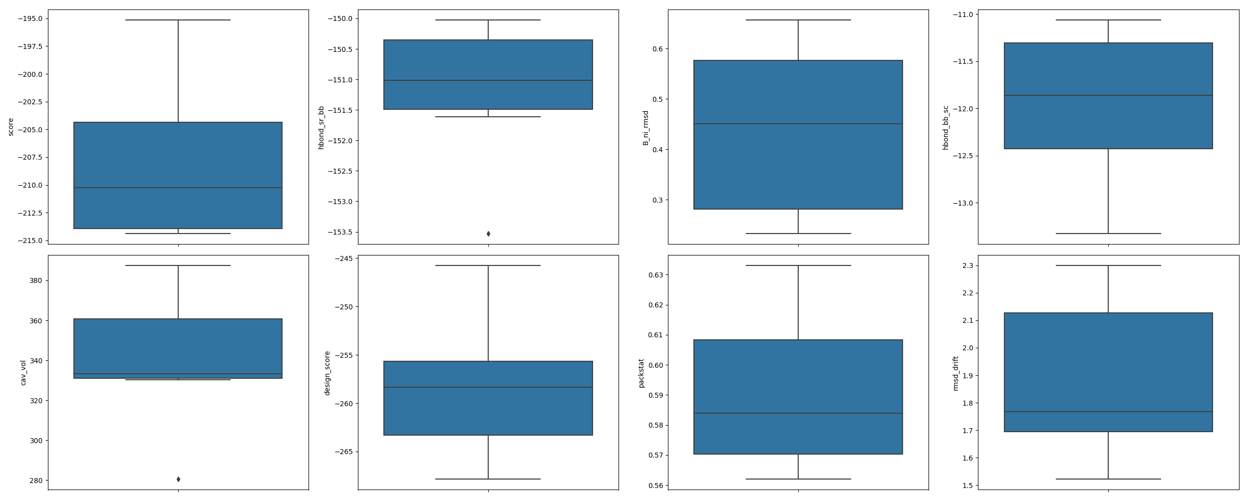
In [1]: from rstoolbox.io import parse_rosetta_file
   ...: from rstoolbox.plot import multiple_distributions
   ...: import matplotlib.pyplot as plt
   ...: df = parse_rosetta_file("../rstoolbox/tests/data/input_2seq.minisilent.gz")
   ...: values = ["score", "hbond_sr_bb", "B_ni_rmsd", "hbond_bb_sc",
   ...:           "cav_vol", "design_score", "packstat", "rmsd_drift"]
   ...: fig = plt.figure(figsize=(25, 10))
   ...: axs = multiple_distributions(df, fig, (2, 4), values=values)
   ...: plt.tight_layout()
   ...: 

In [2]: plt.show()

In [3]: plt.close()

../_images/multiple_distributions_docs.png

Example 2: Design population data vs. DB reference.

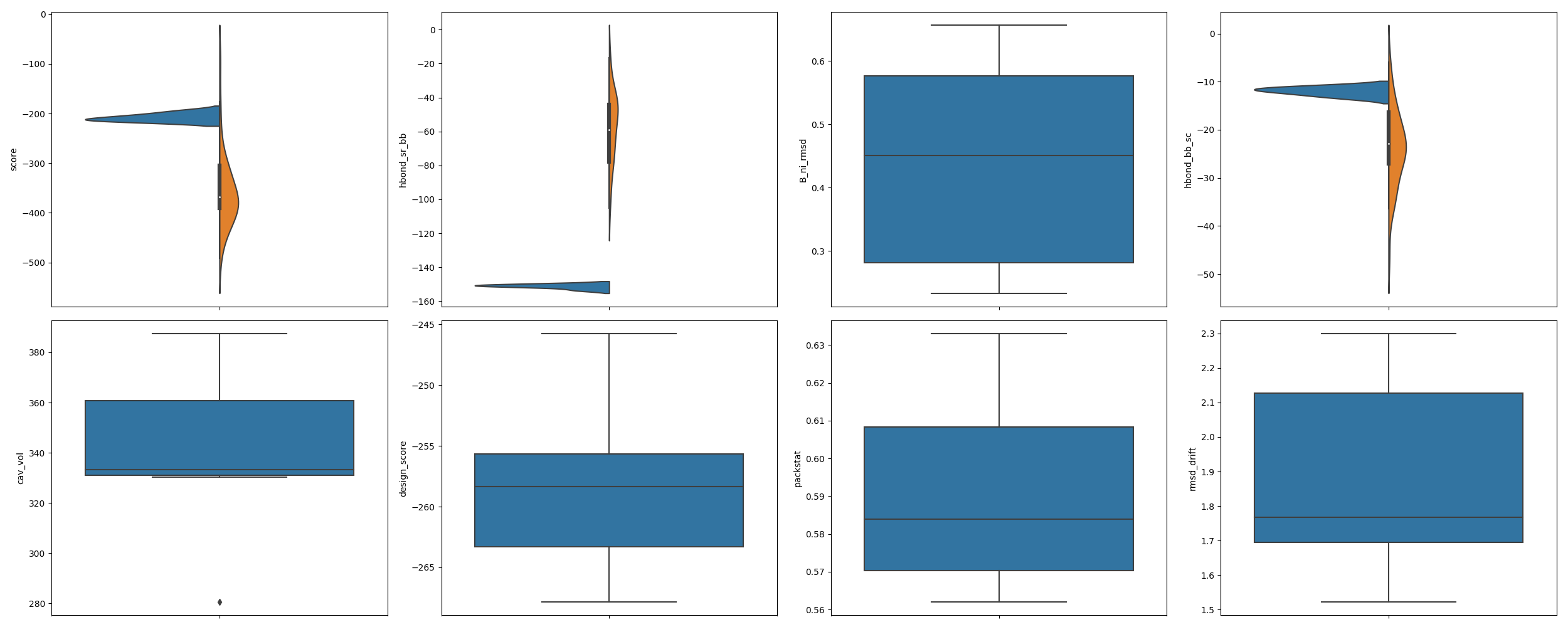
In [4]: from rstoolbox.io import parse_rosetta_file
   ...: from rstoolbox.plot import multiple_distributions
   ...: from rstoolbox.utils import load_refdata
   ...: import matplotlib.pyplot as plt
   ...: df = parse_rosetta_file("../rstoolbox/tests/data/input_2seq.minisilent.gz",
   ...:                         {'sequence': 'A'})
   ...: slength = len(df.iloc[0]['sequence_A'])
   ...: refdf = load_refdata('scop2')
   ...: refdf = refdf[(refdf['length'] >= slength - 5) &
   ...:               (refdf['length'] <= slength + 5)]
   ...: values = ["score", "hbond_sr_bb", "B_ni_rmsd", "hbond_bb_sc",
   ...:           "cav_vol", "design_score", "packstat", "rmsd_drift"]
   ...: fig = plt.figure(figsize=(25, 10))
   ...: axs = multiple_distributions(df, fig, (2, 4), values=values, refdata=refdf)
   ...: plt.tight_layout()
   ...: 

In [5]: plt.show()

In [6]: plt.close()

../_images/multiple_distributions_docs2.png