Structural Analysis
Structural data can be obtained in multiple ways, and it should be relatively easy to implement a DSSP or PSIPRED parser to include that data into the decoy population.
In line of a Rosetta pipeline, the easiest way is to include the WriteSSEMover into a RosettaScript. This could even be called from inside the library as explained in Sequence Analysis.
Loading a Reference
As in Sequence Analysis, we will need to load a reference with get_sequence_and_structure().
Note
Through all the process several times the chainID of the decoy of interest will be called. This is due to the fact that the library can manipulate
decoys with multiple chains (designed or not), and, thus, analysis must be called upon the sequences of interest.
In [1]: import rstoolbox as rs
   ...: import pandas as pd
   ...: import matplotlib.pyplot as plt
   ...: import seaborn as sns
   ...: plt.rcParams['svg.fonttype'] = 'none' # When plt.savefig to 'svg', text is still text object
   ...: sns.set_style('whitegrid')
   ...: pd.set_option('display.width', 1000)
   ...: pd.set_option('display.max_columns', 500)
   ...: pd.set_option("display.max_seq_items", 3)
   ...: baseline = rs.io.get_sequence_and_structure('../rstoolbox/tests/data/2pw9C.pdb')
   ...: baseline.get_structure('C')
   ...:
Out[1]:
0    LEEEEEEELLEEEEEEEELLLLHHHHHHHHHHHHLLLLLLLLLLLEEEELLLEEEELL
Name: structure_C, dtype: object
Loading the Design Data
Again, we are mimicking Sequence Analysis, but in this case we load the structural data of the designs along with their dihedrals.
In [2]: rules = {'scores_ignore': ['fa_*', 'niccd_*', 'hbond_*', 'lk_ball_wtd', 'pro_close', 'dslf_fa13', 'C_ni_rmsd_threshold',
   ...:                            'omega', 'p_aa_pp', 'yhh_planarity', 'ref', 'rama_prepro', 'time'],
   ...:          'sequence': 'C', 'structure': 'C', 'dihedrals': 'C',
   ...:          'labels': ['MOTIF', 'SSE03', 'SSE05']}
   ...: df = rs.io.parse_rosetta_file('../rstoolbox/tests/data/input_ssebig.minisilent.gz', rules)
   ...: df.add_reference_structure('C', baseline.get_structure('C'))
   ...: df.add_reference_shift('C', 32)
   ...: df.head(3)
   ...:
Out[2]:
    score  ALIGNRMSD  BUNS  COMPRRMSD  C_ni_mtcontacts  C_ni_rmsd  C_ni_trials  MOTIFRMSD  cav_vol  driftRMSD  finalRMSD  packstat C_ni_rmsd_type                            description lbl_MOTIF lbl_SSE03 lbl_SSE05                                                  sequence_C                                                 structure_C                           phi_C                             psi_C
0 -64.070  0.608      12.0  7.585      4.0              3.301      1.0          0.957      66.602   0.083      3.323      0.544     no_motif       nubinitio_wauto_18326_2pw9C_0001_0001  [C]       [C]       [C]       TTWIKFFAGGTLVEEFEYSSVNWEEIEKRAWKKLGRWKKAEEGDLMIVYPDGKVVSWA  LEEEEEEELLLEEEEEEELLLLHHHHHHHHHHHHLLLLLLLLLLLEEEELLLEEEELL  [0.0, -143.01, -92.3838, ...]   [163.023, 142.263, 136.923, ...]
1 -70.981  0.639      12.0  2.410      8.0              1.423      1.0          0.737      0.000    0.094      1.395      0.552     no_motif       nubinitio_wauto_18326_2pw9C_0002_0001  [C]       [C]       [C]       NTWSTNILNGHPKITLLVEERGAEEIHLEWLKKQGLRKKAEENVYTTKLPNGAVKVYG  LEEEEEEELLEEEEEEEELLLLHHHHHHHHHHHLLLLLLLLLLLEEEELLLLLEEEEL  [0.0, -144.628, -82.9913, ...]  [109.954, 146.837, 129.948, ...]
2 -43.863  0.480      8.0   4.279      6.0              2.110      1.0          0.819      93.641   0.110      2.106      0.575     no_motif       nubinitio_wauto_18326_2pw9C_0003_0001  [C]       [C]       [C]       PRWFIAMGDGVIWEIVLGSEQNLEEIAKKGLKRRGLYKKAEESIYTIIYPDGIAHTFG  LEEEEEEELLEEEEEEEELLLLHHHHHHHHHHHHLLLLLLLLLLEEEEELLLEEEEEL  [0.0, -143.373, -78.9875, ...]  [141.285, 139.737, 129.8, ...]
Select by Structural Properties
One of the most obvious assessments is the calculation of percentages of secondary structure. We can even use that to pre-select decoys. For example,
let’s assume that we want to make sure that strand 5 (SSE05) from the selected labels is mostly still a strand after our design protocol:
In [3]: sse05 = df.get_label('SSE05', 'C').values[0]
   ...: df = rs.analysis.secondary_structure_percentage(df, 'C', sse05)
   ...: dfsse = df[df['structure_C_E'] > 0.8]
   ...: dfsse.head(3)
   ...:
Out[3]:
    score  ALIGNRMSD  BUNS  COMPRRMSD  C_ni_mtcontacts  C_ni_rmsd  C_ni_trials  MOTIFRMSD  cav_vol  driftRMSD  finalRMSD  packstat C_ni_rmsd_type                            description lbl_MOTIF lbl_SSE03 lbl_SSE05                                                  sequence_C                                                 structure_C                           phi_C                             psi_C  structure_C_H  structure_C_E  structure_C_L
2 -43.863  0.480      8.0   4.279      6.0              2.110      1.0          0.819      93.641   0.110      2.106      0.575     no_motif       nubinitio_wauto_18326_2pw9C_0003_0001  [C]       [C]       [C]       PRWFIAMGDGVIWEIVLGSEQNLEEIAKKGLKRRGLYKKAEESIYTIIYPDGIAHTFG  LEEEEEEELLEEEEEEEELLLLHHHHHHHHHHHHLLLLLLLLLLEEEEELLLEEEEEL  [0.0, -143.373, -78.9875, ...]  [141.285, 139.737, 129.8, ...]    0.0            0.833333       0.166667
3 -75.847  0.454      7.0   3.112      8.0              1.746      1.0          1.629      39.232   0.083      1.734      0.644     no_motif       nubinitio_wauto_18326_2pw9C_0004_0001  [C]       [C]       [C]       PYEWVFIINGVPQTTWNHPPTKMEELEKFARKKGGSSKKAEEGKFAIIIWKGYFIVSD  LLLEEEEELLEEEEEELLLLLLHHHHHHHHHHHHLLLLLLLLLLEEEEELLLEEEEEL  [0.0, -130.948, -160.432, ...]  [141.392, 174.651, 115.305, ...]  0.0            0.833333       0.166667
6 -47.169  0.430      6.0   3.313      6.0              2.050      1.0          0.641      0.000    0.112      1.975      0.551     no_motif       nubinitio_wauto_18326_2pw9C_0007_0001  [C]       [C]       [C]       PREWEGRYNGVPRGREWALPTNLEELMKEMRKRAGGYKKAEEGIYATIFPNGVILVRG  LEEEEEEELLEEEEEEEELLLLHHHHHHHHHHHHLLLLLLLLLLEEEEELLLEEEEEL  [0.0, -133.286, -93.7573, ...]  [142.271, 153.259, 120.778, ...]  0.0            0.833333       0.166667
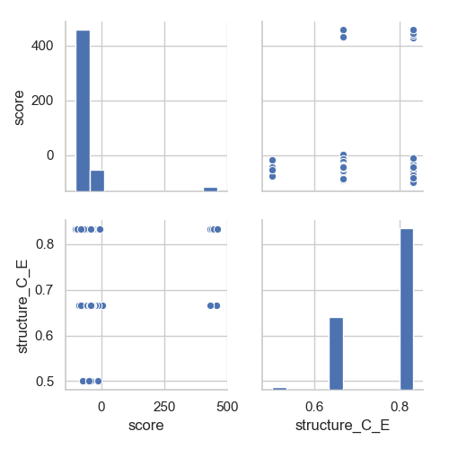
Or that we want to check if there is a correlation between the final score of our decoys and the level of conservation of strand 5 (which does not seem to be the case):
In [4]: grid = sns.pairplot(df[['score', 'structure_C_E']])

In [5]: plt.show()
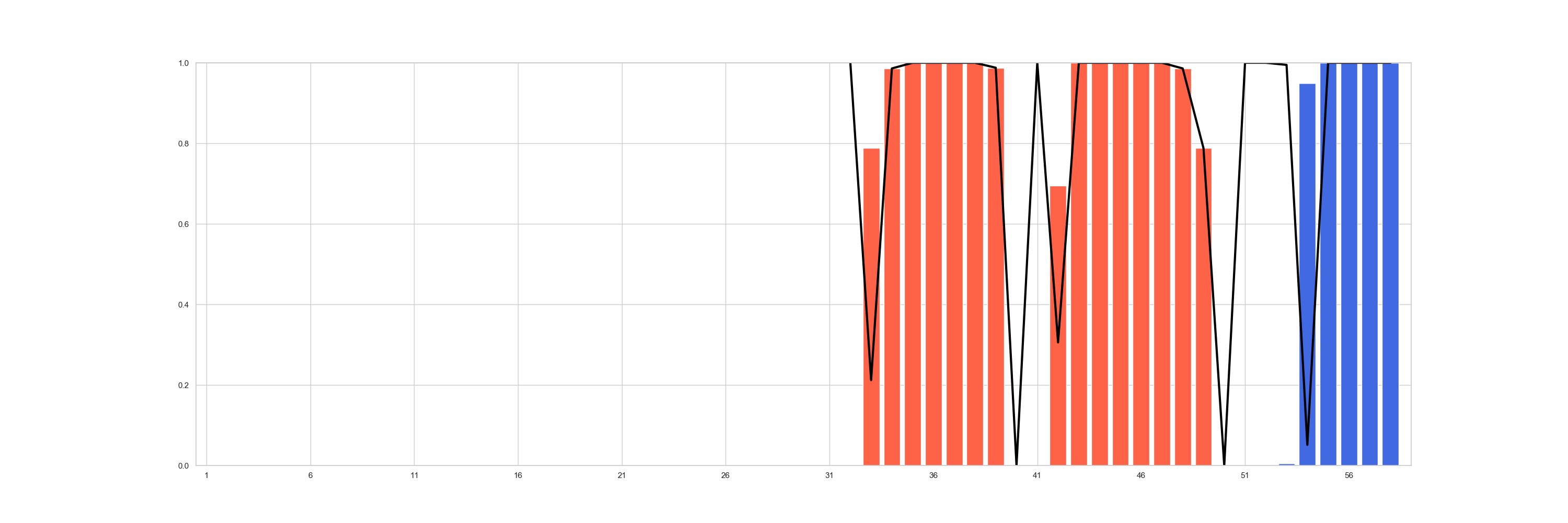
Visualise Structural Data
The most global view, would be to see for all the population how often the expected secondary structure is retrieved with
positional_structural_similarity_plot().
In [6]: fig  = plt.figure(figsize=(30, 10))
   ...: ax = plt.subplot2grid((1, 1), (0, 0))
   ...: sseid1 = rs.analysis.positional_structural_count(df, 'C')
   ...: sseid2 = rs.analysis.positional_structural_identity(df, 'C')
   ...: rs.plot.positional_structural_similarity_plot(pd.concat([sseid1, sseid2], axis=1), ax)
   ...:

In [7]: plt.show()
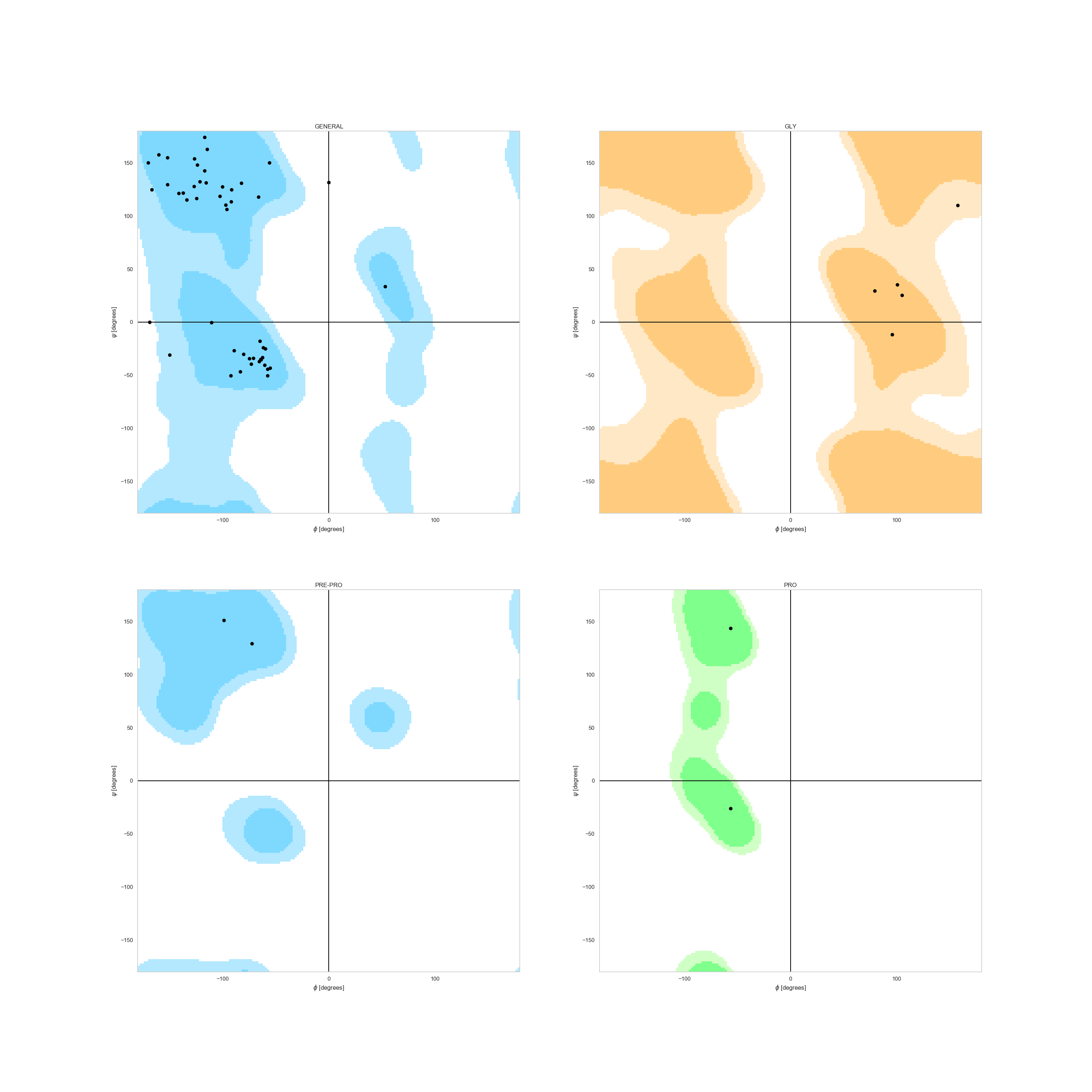
In case of a single decoy, and thanks to our request for dihedrals in the parsing rules, we can check whether or not
a the decoy’s Ramachandran Plot makes sense. We can observe it, for example, for the best
scored decoy under the plot_ramachandran() function.
Note
Dihedral angles are also obtained through WriteSSEMover,
but they can easily be added by parsing them into a list and adding them to the DesignFrame with the column name psi_<seqID> and phi_<seqID>.
In [8]: fig  = plt.figure(figsize=(30, 30))
   ...: _ = rs.plot.plot_ramachandran(df.sort_values('score').iloc[0], 'C', fig)
   ...:

In [9]: plt.show()
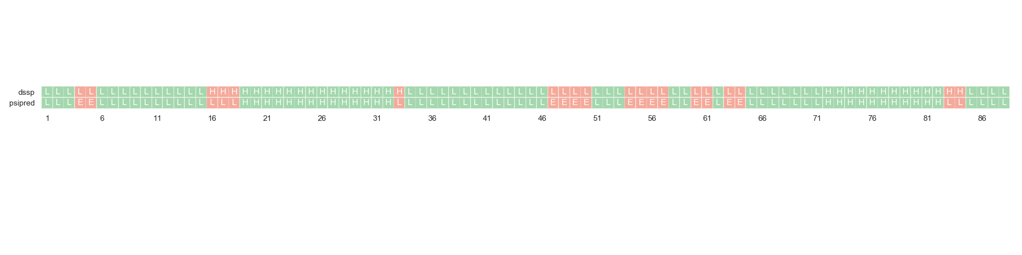
Finally, one can compare the actual DSSP assignation against PSIPRED’s sequence-based secondary structure prediction. This can give an idea of the feasibility of the sequence to actually fold in the expected conformation.
For this, we are going to load a different dataset in which this data is present.
In [10]: fig = plt.figure(figsize=(20, 5))
   ....: rules = {"scores": ["score"], "psipred": "*", "structure": "*", "dihedrals": "*" }
   ....: df2 = rs.io.parse_rosetta_file("../rstoolbox/tests/data/input_3ssepred.minisilent.gz", rules)
   ....: ax = plt.subplot2grid((1, 1), (0, 0))
   ....: rs.plot.plot_dssp_vs_psipred(df2.iloc[0], "A", ax)
   ....: plt.tight_layout()
   ....: fig.subplots_adjust(top=1.2)
   ....:

In [11]: plt.show()

In [12]: plt.close('all')