Contextualize your Data
The generation of a new design population can provide a lot of data depending in the number of filters and metrics used to evaluate them. Still, although these scores allow for the sorting and selection of decoys of interest, it does not always provide a comprehensive analysis of that population with regard to the general population of known protein structures.
The rstoolbox provides some helper functions and datasets in order to properly assess this issue.
Pre-calculated datasets
There is a total of 4 different pre-calculated datasets that can be loaded directly with the rstoolbox; those are cath, scop,
scop2 and chain (for PDB chains). For this datasets, homology (as provided by the PDB database) can be used to avoid over-represented
structures. The access to these datasets is provided through the load_refdata() function:
In [1]: import rstoolbox as rs
   ...: import pandas as pd
   ...: import matplotlib.pyplot as plt
   ...: import seaborn as sns
   ...: plt.rcParams['svg.fonttype'] = 'none' # When plt.savefig to 'svg', text is still text object
   ...: sns.set_style('whitegrid')
   ...: pd.set_option('display.width', 1000)
   ...: scop2 = rs.utils.load_refdata('scop2')
   ...: scop2_70 = rs.utils.load_refdata('scop2', 70)  # 70% homology filter
   ...: scop2_70.drop(columns=['sequence_$', 'structure_$', 'psi_$', 'phi_$', 'node_name']).head(5)
   ...:
Out[1]:
   scop_id  serial   pdb chain  begin  end   selectors  leaf      domain_id    score  hbond_sr_bb  hbond_lr_bb  hbond_bb_sc  hbond_sc  dslf_fa13   omega  p_aa_pp  yhh_planarity      ref  rama_prepro  BUNS  CYDentropy  avdegree  beta  breaks   cavity  charge  exposed_hyd  helix  long_apolar  long_polar   pack  psipred  radius  length                                        node_id
0  8003767  1       2UWE  I     1      99   (I:1-99,)   True  2UWEI80037671 -237.172 -8.136       -42.638      -17.730      -7.007    -1.163      9.673  -23.884   0.026          8.637   -8.386        2.0   7.735       10.010    6.0   0.0     10.279  -2.0     932.371      0.0    6.0          6.0         0.661  0.727    14.066  99      [2000051, 6001103, 5000763, 4000202, 3000071]
1  8003798  1       2OAN  C     4      371  (C:4-371,)  True  2OANC80037981 -898.795 -139.883     -78.118      -37.999      -39.343    0.000      33.758 -72.597   0.036          121.341  2.231        31.0  0.000       11.330    13.0  1.0     294.330 -12.0    2812.701     15.0   7.0          6.0         0.657  0.675    21.333  357     [3000092, 6001267, 5000898, 4000313]
2  8003706  1       2UUB  M     2      125  (M:2-125,)  True  2UUBM80037061 -74.236  -56.345      -4.286       -7.571       -5.800     0.000      6.343  -22.039   0.001          43.878   10.694       17.0  0.000       9.516     0.0   0.0     41.054   19.0    1472.719     6.0    6.0          8.0         0.631  0.758    21.976  124     [6001039, 5000712, 4000260]
3  8017549  1       1FQB  A     2      370  (A:2-370,)  True  1FQBA80175491 -957.723 -144.574     -69.207      -53.420      -29.550    0.000      15.504 -71.976   0.045          83.748   4.174        42.0  0.000       11.715    12.0  0.0     432.225 -9.0     2157.583     16.0   8.0          5.0         0.671  0.702    21.546  369     [6002815, 5001965]
4  8004502  1       1W8M  A     2      164  (A:2-164,)  True  1W8MA80045021 -461.079 -36.431      -56.442      -37.828      -15.055    0.000      17.157 -58.100   0.004          57.392  -3.910        17.0  0.000       11.294    8.0   0.0     38.591   2.0     1157.008     2.0    7.0          10.0        0.786  0.687    14.256  163     [6001369, 5000991, 4000390, 3000168, 2000164]
These sets are only provided as help, but the user can create its own sets, as long as they are loaded as a DataFrame.
Cleaning your own background sets
In case one has its own background reference dataset, rstoolbox offers the option to retrieve homology clusters precalculated
from PDB with the make_redundancy_table() function. By default, this function will call on the PDB’s ftp to download those
homology cluster files, but with precalculated==True it will directly provide a quicker access to the table available in the
library (as the first option is relatively time consuming).
The generated table can be used on your reference set as long as a pdb and chain column exists.
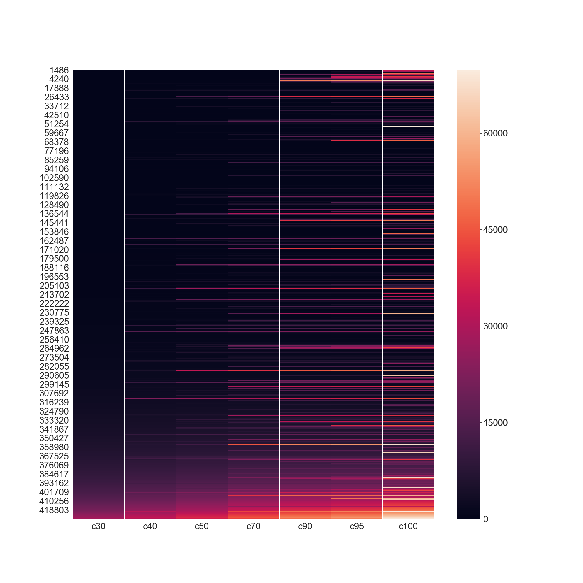
The following example shows now this table can be applied in what would be the equivalent of rs.utils.load_refdata('scop2', 30)
and creates a visual representation of the clusters.
In [2]: hmdf = rs.utils.make_redundancy_table(precalculated=True)
   ...: scop2_30 = scop2.merge(hmdf, on=['pdb', 'chain'])
   ...: scop2_30 = scop2_30.sort_values('score').groupby('c30').first().reset_index()
   ...: fig = plt.figure(figsize=(20, 20))
   ...: ax = plt.subplot2grid((1, 1), (0, 0), fig=fig)
   ...: _ = sns.heatmap(hmdf.drop(columns=['pdb', 'chain']).sort_values(['c30', 'c40', 'c50', 'c70', 'c90', 'c95', 'c100']), ax=ax)
   ...:

In [3]: plt.show()
Distribution in context
Let’s assume the following population dataset:
In [4]: rules = {'scores_ignore': ['fa_*', 'niccd_*', 'hbond_*', 'lk_ball_wtd', 'pro_close', 'dslf_fa13', 'C_ni_rmsd_threshold',
   ...:                            'omega', 'p_aa_pp', 'yhh_planarity', 'ref', 'rama_prepro', 'time'],
   ...:          'sequence': 'C',
   ...:          'labels': ['MOTIF', 'SSE03', 'SSE05']}
   ...: df = rs.io.parse_rosetta_file('../rstoolbox/tests/data/input_ssebig.minisilent.gz', rules)
   ...: df.head(3)
   ...:
Out[4]:
    score  ALIGNRMSD  BUNS  COMPRRMSD  C_ni_mtcontacts  C_ni_rmsd  C_ni_trials  MOTIFRMSD  cav_vol  driftRMSD  finalRMSD  packstat C_ni_rmsd_type                            description lbl_MOTIF lbl_SSE03 lbl_SSE05                                                  sequence_C
0 -64.070  0.608      12.0  7.585      4.0              3.301      1.0          0.957      66.602   0.083      3.323      0.544     no_motif       nubinitio_wauto_18326_2pw9C_0001_0001  [C]       [C]       [C]       TTWIKFFAGGTLVEEFEYSSVNWEEIEKRAWKKLGRWKKAEEGDLMIVYPDGKVVSWA
1 -70.981  0.639      12.0  2.410      8.0              1.423      1.0          0.737      0.000    0.094      1.395      0.552     no_motif       nubinitio_wauto_18326_2pw9C_0002_0001  [C]       [C]       [C]       NTWSTNILNGHPKITLLVEERGAEEIHLEWLKKQGLRKKAEENVYTTKLPNGAVKVYG
2 -43.863  0.480      8.0   4.279      6.0              2.110      1.0          0.819      93.641   0.110      2.106      0.575     no_motif       nubinitio_wauto_18326_2pw9C_0003_0001  [C]       [C]       [C]       PRWFIAMGDGVIWEIVLGSEQNLEEIAKKGLKRRGLYKKAEESIYTIIYPDGIAHTFG
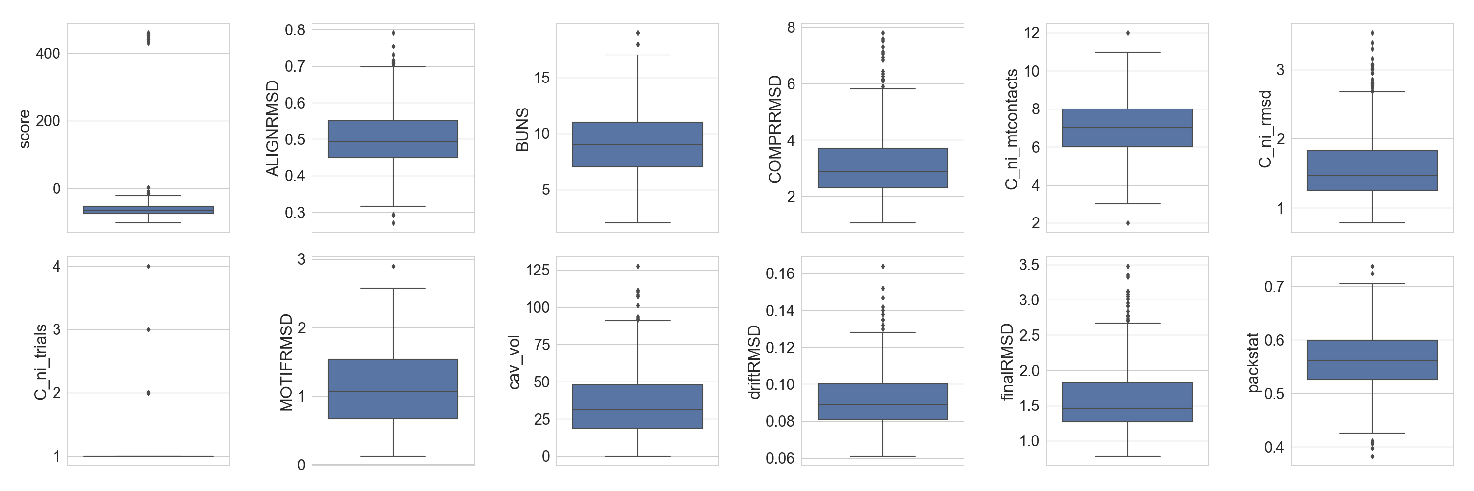
As previously demonstrated in the sequence analysis tutorial, we can preview the distribution of different scores of the design population:
In [5]: fig  = plt.figure(figsize=(30, 10))
   ...: grid = [2, 6]
   ...: axes = rs.plot.multiple_distributions( df, fig, grid )
   ...: plt.tight_layout()
   ...:

In [6]: plt.show()
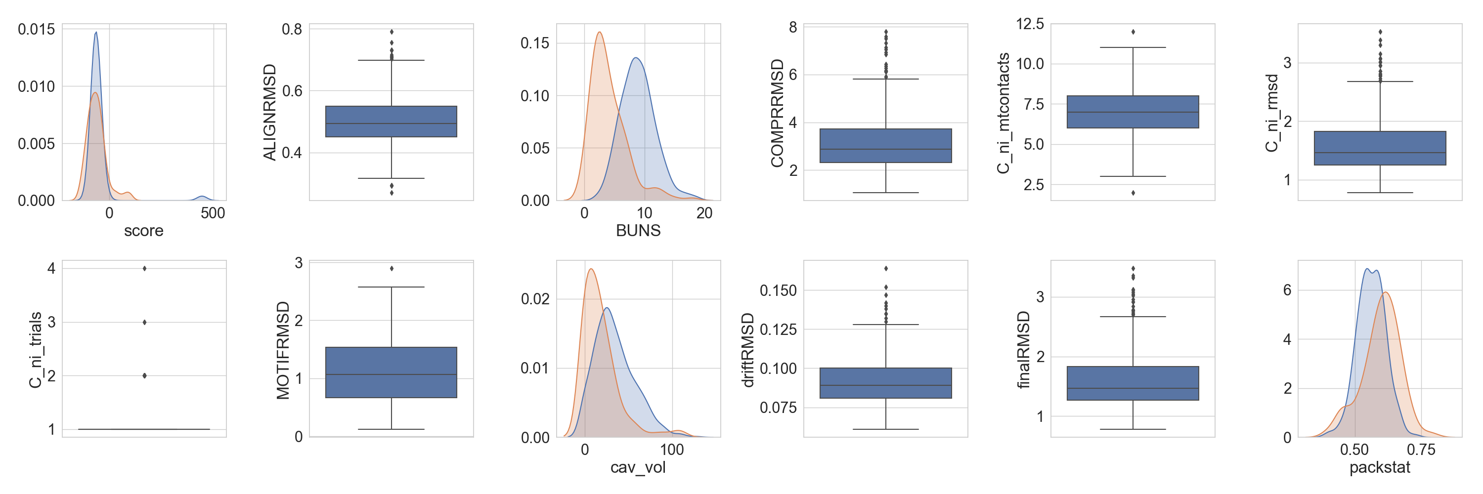
But we can also see the population behave against other protein of a similar size.
Note
The function will pick up that columns with the same name are the same, for others that should be the same but are called
differently, a translation dictionary can be provided, as is the case in this example with cavity volume and packstat
data.
In [7]: slength = len(df.iloc[0].get_sequence('C'))
   ...: refdf = scop2[(scop2['length'] >= slength - 5) &
   ...:               (scop2['length'] <= slength + 5) &
   ...:               (scop2['score'] <= 100)]
   ...: fig = plt.figure(figsize=(30, 10))
   ...: axs = rs.plot.multiple_distributions(df, fig, grid, refdata=refdf, violins=False,
   ...:                                      ref_equivalences={'cavity': 'cav_vol', 'pack': 'packstat'})
   ...: plt.tight_layout()
   ...:

In [8]: plt.show()
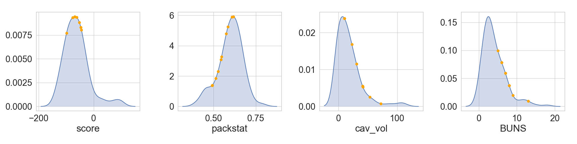
Selections in context
Contrary to the previous example, in which full distributions where compared, another useful tool is the ability to place selected structures in a given context. This can have two main uses: (1) see the position of selected decoys in a given distribution or (2) see the quality of putative template scaffolds before working with them.
In [9]: pickdf = df.sample(10)
   ...: fig = plt.figure(figsize=(20, 5))
   ...: axs = rs.plot.plot_in_context(pickdf, fig, (1, 4), refdata=refdf, values= ['score', 'packstat', 'cav_vol', 'BUNS'],
   ...:                               ref_equivalences={'cavity': 'cav_vol', 'pack': 'packstat'})
   ...: plt.tight_layout()
   ...:

In [10]: plt.show()
Each selection in its context
Multiple selected decoys or scaffolds originated from different sources might not be all comparable under the same set. The most simple case would be when those structures do not have a similar length, which does affect Rosetta scores. In those scenarios, it is possible to see, for each decoy of interest, how well it compares to its reference dataset, and rank them according to which quantile of the distribution they belong to:
In [11]: df = rs.utils.load_refdata('scop')
   ....: qr = pd.DataFrame([['2F4V', 'C'], ['3BFU', 'B'], ['2APJ', 'C'],
   ....:                    ['2C37', 'V'], ['2I6E', 'H']], columns=['pdb', 'chain'])
   ....: qr = qr.merge(df, on=['pdb', 'chain'])
   ....: refs = []
   ....: for i, t in qr.iterrows():
   ....:   refs.append(df[(df['length'] >= (t['length'] - 5)) &
   ....:                  (df['length'] <= (t['length'] + 5))])
   ....: fig  = plt.figure(figsize=(22, 7))
   ....: rs.plot.distribution_quality(df=qr, refdata=refs,
   ....:                              values=['score', 'pack', 'avdegree', 'cavity', 'psipred'],
   ....:                              ascending=[True, False, True, True, False],
   ....:                              names=['domain_id'], fig=fig)
   ....: plt.tight_layout()
   ....:

In [12]: plt.show()